Dense matter QFT with the DS L=24 1e-08 LLR L=24 O( ) DS L=22 - - PowerPoint PPT Presentation

Dense matter QFT with the density-of-states method

Kurt Langfeld, Centre of Mathematical Sciences, Plymouth University Sign 2015, Institute for Nuclear Research, Debrecen, 1st October 2015

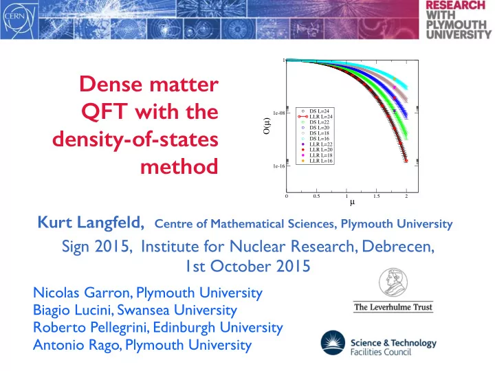
0.5 1 1.5 2

µ

1e-16 1e-08 1

O(µ)

DS L=24 LLR L=24 DS L=22 DS L=20 DS L=18 DS L=16 LLR L=22 LLR L=20 LLR L=18 LLR L=16

Nicolas Garron, Plymouth University Biagio Lucini, Swansea University Roberto Pellegrini, Edinburgh University Antonio Rago, Plymouth University

Overview:

What do we know about QFTs with a sign problem? Promising algorithmic attempts [Complex Langevin, Lefschetz Thimble, strong coupling

methods, ….] Here: density-of-states method, dualisation (bench marking)

Foundations of the LLR-approach [the U(1) showcase] Can we solve a strong sign problem with the LLR method? [yes! Theory & the Z3 showcase]

Overview:

Anatomy of a sign problem: Heavy-Dense QCD (HDQCD) Theory: particle-hole duality the Inverse-Silver-Blaze feature [new physics?] Results from re-weighting [regions of strong-sign-problem] Results from the density-of-states approach (LLR method)

Phases of QCD

What did we know in 2003 from 1st principles?

D’

What do we know NOW from 1st principles?

D’

What do we NOT know from 1st principles?

chiral spirals

What is the problem?

How can we quantify the problem?

If we drop the imaginary part of the action:

ZPQ(µ) = Z Dφ exp{SR[φ]}

Define the overlap between full and phase quenched theory

O(µ) = Z(µ) ZPQ(µ) = hexp{iµSI}iPQ

Standard re-weighting: standard MC

hAi = hA exp{iSI}iPQ h exp{iSI}iPQ

Overlap problem:

depends on only for:

Silver Blaze Problem:

[low temperatures, large volumes]

Z(µ) µ µ > mthreshold

not satisfied by ZPQ(µ) !

[Tom Cohen, 2003]

and have different free energy densities

Z ZPQ O(µ) = Z(µ) ZPQ(µ) = exp{−∆f V } ⇒ can be very small

re-weighting is inefficient!

(∆f > 0)

…and a simple, but important identity:

Recall the definition of the density: ρ(µ) = T

V3 ∂ ln Z(µ) ∂µ

Trivially:

Z(µ) = Z(µ) ZPQ(µ) ZPQ(µ) = O(µ) ZPQ(µ)

Silver Blaze Problem

µ < mthreshold > 0 neglectet ρ(µ) = T V3 ∂ ∂µ ln O(µ) + ρPQ(µ)

Promising attempts to solve QFTs with sign problems:

[this is not a complete list!]

LLR Approach

Wang-Landau type algorithm: Target: density-of-states Partition function:

Z = Z dE ρ(E) exp{βE}

1. Divide action range in intervals 2. Generate configurations for each interval 3. Generate action histogram

Wang-Landau type algorithm:

4. Include as re-weighting factor 5. re-fine until histogram is flat 6. patch together the from intervals to the overall density

ρ−1 ρ

Advantage: solves overlap problems!

[Wang, Landau, PRL 86 (2001) 2050]

Ideal for systems with discrete action range (spin systems)

ρ

Disadvantage: histogram edge effects for continuous systems

LLR approach:

For small enough : Poisson distribution

δE

restriction to the action range re-weighting factor

• bservable

need to find “a” !

standard MC average

h hW[φ]i ik(a) = 1 Nk Z Dφ θ[Ek,δE](S[φ]) W[φ] e−aS[φ]

LLR approach:

Choose: h h∆Ei ik(a) ∆E = S[φ] − Ek − δE/2 If “a” is correct, the distribution is flat implying = 0 non-linear stochastic equation Use e.g. Newton Raphson to solve for “a”:

[Langfeld, Lucini, Rago, PRL 109 (2012) 111601]

an+1 = an + 12 δE2 h h∆Ei i (an)

LLR approach:

[Langfeld, Lucini, Rago, PRL 109 (2012) 111601]

Reconstruct the density-of-states:

N(E) : EN ≤ E < EN+1 ρ(E) = ρ0 N−1 Y

k=1

eakδE ! eaN(E−EN)

Features:

• 2nd order accuracy:
• Exponential error suppression !

O(δE2)

[Langfeld, Lucini, Pellegrini, Rago, arXiv:1509.08391]

LLR approach: Indicative result:

SU(2) & SU(3) gauge theories Emax = 60, 000

h h∆Ei ik(a)

LLR approach: Technical progress:

Different versions of the iteration might improve convergence

a(n+1) = a(n) +

h h∆Ei ik(a(n)) σ2(∆E;a(n)) [Gattringer, Toerek, PLB 747 (2015) 545]

Solving the stochastic equation: Statistical noise interferes with convergence a(n+1) = a(n) +

1 max(n−nth,1) 12 δE2 h

h∆Ei ik (a(n)) Robbins-Monro (1951) under-relaxation: converges to the true solution “a”!

[Pellegrini, Langfeld, Lucini, Rago, PoS LATTICE2014 (2015) 229]

LLR approach: Early objections

• 1. Is the LLR approach ergodic?

Use the Replica Exchange method: Use the LLR estimate for as re-weighting factor ρ R Dφ ρ−1(S[φ) W[φ] ρ(S[φ) eβS random walk in configuration space

• bservable

[Langfeld, Lucini, Pellegrini, Rago, arXiv:1509.08391]

Yes!

LLR approach: Indicative result for U(1) (more later)

1.006 1.008 1.01 1.012 1.014

β

0.6 0.61 0.62 0.63 0.64 0.65 0.66 0.67

〈E〉

LLR Multicanonical

[Langfeld, Lucini, Pellegrini, Rago, arXiv:1509.08391] (credits to RP & AR)

LLR approach: Early objections

• 2. You can only calculate observables that are a

function of S[φ]

Typically: hSni =

R dE En ρ(E) eβE R dEρ(E) eβE

Progress: arbitrary observables accessible

hB[φ]i =

1 Z(β)

P

i δE ˜

ρ (Ei) h hB[φ] exp{βS[φ] + ai(S[φ] Ei)}i i

Z(β) = P

i δE ˜

ρ (Ei) h hexp{βS[φ] + ai(S[φ] Ei)}i i

2nd order accuracy: O(δE2) [same of for the density-of-states]

[Langfeld, Lucini, Pellegrini, Rago, arXiv:1509.08391]

…enough theory. We want results!

LLR approach

4d compact U(1) gauge theory

Record: lattice, multicanonical HMC + supercomputer 184 Theory with a (very) weak 1st order phase transition

[Arnold, Lippert,Neuhaus, Schilling, Nucl.Phys.Proc.Suppl. 94 (2001) 651]

LLR: how does a(E) depend on the lattice size? expectation: a = d ln ρ

dE [independent of L for large L]

0.58 0.6 0.62 0.64 0.66 0.68

ε

• 1.04
• 1.02
• 1

ai L=8 L=10 L=12 L=14 L=16 L=18 L=20

LLR approach

4d compact U(1) gauge theory

How does the LLR results compare with those from the literature? Define critical coupling from the peak position of the specific heat βc(L) record!

(credits to RP & AR)

LLR approach

4d compact U(1) gauge theory

The probability distribution for : ρ(E) eβE β = βc(∞)

L=20

0.61 0.62 0.63 0.64 0.65 0.66 0.67

E/6V

20 40 60 80 100 120

Pβ(E)

LLR approach

4d compact U(1) gauge theory

Do we achieve the predicted precision ? O(δE2) The specific heat: cV (βc(L))

0.02 0.04 0.06 0.08 δE/V 2.0e-04 3.0e-04 4.0e-04 5.0e-04 6.0e-04 CV(βc(L)) L=8 L=10 L=12 L=14 L=16

yes!

The LLR algorithm is designed to solve overlap problems, but can it solve Sign problems?

Recall: theory with complex action

Define the generalised density-of-states: Partition function emerges from a FT:

LLR approach for complex systems:

Need to calculate the overlap density, etc O(µ) = Z(µ) ZPQ(µ) = R ds exp{iµs} Pβ(s) R ds Pβ(s)

• verall normalisation drops out

Testbed: Z3 Polyakov line model (3d spin model, discrete) τ : temperature, η = κ eµ , ¯ η = κ e−µ z ∈ Z3 Solvable: dual theory is real, efficient flux algorithm

[Mercado, Evertz, Gattringer, PRL 106 (2011) 222001]

Z3 spin model

Dual solutions show: Strong sign problem

snake algorithm

LLR approach:

Z3 spin model

What is the challenge [without dualisation]? Indicative result:

action volume statistical errors exponentially small Need exponential error suppression over the whole action range

LLR approach:

Z3 spin model

Numerical findings

• 1000

1000 2000 3000 4000 5000 6000

N+ - N-

1e-60 1e-45 1e-30 1e-15 1 histogram density-of-states

Pβ(s) s = needed for FT

[Langfeld, Lucini, PRD 90 (2014) 094502]

LLR approach:

Z3 spin model

Numerical findings

[Langfeld, Lucini, PRD 90 (2014) 094502]

We haven’t talked about FT (see later), but our findings are:

0.5 1 1.5 2

µ

1e-16 1e-08 1

O(µ)

DS L=24 LLR L=24 DS L=22 DS L=20 DS L=18 DS L=16 LLR L=22 LLR L=20 LLR L=18 LLR L=16

First “head on” solution of a sign problem!

Z3 spin model

Silver Blaze Problem in the Z3 model: Recall: always negative The phase quenched theory always overestimates the true density ρ(µ) = T V3 ∂ ∂µ ln O(µ) + ρPQ(µ)

….let’s discuss new physics!

Anatomy of a sign problem: Heavy-Dense QCD (HDQCD) Starting point QCD:

Z(µ) = Z DUµ exp{β SYM[U]} DetM(µ)

SU(3) gauge theory quark determinant

Limit quark mass , large,

m µ

µ/m → finite

[Bender, Hashimoto, Karsch, Linke, Nakamura, Plewnia,

• Nucl. Phys. Proc. Suppl. 26 (1992) 323]

Det M(µ) = Y

~ x

det ⇣ 1 + e(µ−m)/T P(~ x) ⌘2 det ⇣ 1 + e−(µ+m)/T P †(~ x) ⌘2

Low temperatures, :

µ > 0

Det M(µ) = Y

~ x

det ⇣ 1 + e(µ−m)/T P(~ x) ⌘2

neglect anti-quark contribution

Heavy-dense QCD

Limits:

Det M(µ) = Y

~ x

det ⇣ 1 + e(µ−m)/T P(~ x) ⌘2

small: µ

(quenched theory)

DetM(µ) ≈ 1 large: µ DetM(µ) ≈ e3V (µ−m)/T

(saturation)

at threshold: µ

(real, “half-filling”, Hubbard model)

DetM(µ) = Y

~ x

det ⇣ 1 + P(~ x) ⌘2

Is there a sign problem at all?

Heavy-dense QCD

Results from re-weighting

0.4 0.6 0.8 1 1.2 1.4 1.6 1.8 2

µ

0.2 0.4 0.6 0.8 1

< exp (i Φ) >

HDQCD, beta=5.6, kappa=0.12, 8

4

particle - hole duality

[Garron, Langfeld, et al, in preparation] [Rindlisbacher, de Forcrand, arXiv:1509.00087]

sign problem

Heavy-dense QCD

[Garron, Langfeld, et al, in preparation]

low density

0.4 0.6 0.8 1 1.2 1.4 1.6 1.8 2

µ

0.2 0.4 0.6 0.8 1

< exp (i Φ) >

HDQCD, beta=5.6, kappa=0.12, 8

4

“half-filling” saturation

“half-filling” ”µ = m” (physical)

Is QCD real at threshold ?

µ = mB/3

Heavy-dense QCD

0.4 0.6 0.8 1 1.2 1.4 1.6 1.8 2

µ

0.2 0.4 0.6 0.8 1

< exp (i Φ) >

HDQCD, beta=5.6, kappa=0.12, 8

4

[Garron, Langfeld, et al, in preparation] positive derivative

Inverse Silver Blaze feature

Recall:

Phase quenching underestimates the true density!

ρ(µ) = T V3 ∂ ∂µ ln O(µ) + ρPQ(µ)

Heavy-dense QCD

0.4 0.6 0.8 1 1.2 1.4 1.6 1.8 2

µ

0.2 0.4 0.6 0.8 1

< exp (i Φ) >

HDQCD, beta=5.6, kappa=0.12, 8

4

[Garron, Langfeld, et al, in preparation]

LLR approach: Studied two values for µ

benchmarking new results

µ = 1.3321 µ = 1.0621

Heavy-dense QCD

[Garron, Langfeld, et al, in preparation]

LLR approach:

µ = 1.0621

benchmarking

• 0.02
• 0.015
• 0.01
• 0.005

0.005 0.01 0.015 0.02

phase/volume

50 100

probability distribution

histogram LLR SU(3) 8

4, kappa=0.12, beta=5.8, mu = 1.0621

standard histogramming versus LLR approach

Pβ(φ)

Heavy-dense QCD

[Garron, Langfeld, et al, in preparation]

LLR approach:

µ = 1.0621

benchmarking

Pβ(φ)

• 0.02

0.02 0.04 0.06

phase/volume

1e-60 1e-45 1e-30 1e-15 1

probability distribution

histogram LLR SU(3) 8

4, kappa=0.12, beta=5.8, mu = 1.0621

LLR exponential error suppression ! high cumulants

Heavy-dense QCD

LLR approach:

µ = 1.0621

benchmarking How do we calculate the FT?

Remember the overlap: O(µ) = R dφ exp{iφ} Pβ(φ) R dφ Pβ(φ)

is an even function of

Pβ(φ) φ

Polynomial fit:

• find the coefficients (bootstrap)
• do the FT (semi-)analytically
• increase until convergence

ln Pβ(φ) =

p

X

n=0

cn φ2n cn p

[Langfeld, Lucini, PRD 90 (2014) 094502]

Heavy-dense QCD

LLR approach:

µ = 1.0621

benchmarking

2 4 6 8 10 12 14 16

[degree of fit polynomial]/2

0.1 0.125 0.15 0.175 0.2 0.225 0.25

〈 exp{iφ}〉

LLR re-weighting mu=1.0621 kappa=0.12 beta=5.7 8

4 lattice

Acceptable agreement between LLR and re- weighting method

KL preliminary

Heavy-dense QCD

[Garron, Langfeld, et al, in preparation]

LLR approach: new results

standard histogramming versus LLR approach

Pβ(φ)

• 0.04
• 0.02

0.02 0.04 0.06

phase/volume

10 20 30 40 50

probability distribution

histogram LLR SU(3) 8

4, kappa=0.12, beta=5.8, mu = 1.3321

µ = 1.3321

Heavy-dense QCD

[Garron, Langfeld, et al, in preparation]

LLR approach:

Pβ(φ)

LLR exponential error suppression !

new results

• 0.04
• 0.02

0.02 0.04 0.06

phase/volume

1e-09 1e-06 0.001 1

probability distribution

histogram LLR SU(3) 8

4, kappa=0.12, beta=5.8, mu = 1.3321

µ = 1.3321

Heavy-dense QCD

LLR approach: new results How good is the polynomial fit?

µ = 1.3321

0.01 0.02 0.03 0.04 0.05 0.06 0.07

φ/V

• 20
• 15
• 10
• 5

ln Pβ(φ)

LLR data fit: n=6, χ

2/dof = 0.59

SU(3), µ =1.3321, β=5.8, κ=0.12

Heavy-dense QCD

LLR approach: new results convergence?

µ = 1.3321

4 5 6 7 8

[degree of polynom]/2

• 2e-05
• 1e-05

1e-05 2e-05 3e-05 4e-05

O(µ)

SU(3), µ=1.3321, β=5.8, κ=0.12

[KL preliminary]

Preliminary result:

0.13(2) × 10−4

Heavy-dense QCD

LLR approach: new results

µ = 1.3321

0.4 0.6 0.8 1 1.2 1.4 1.6 1.8 2

µ

0.2 0.4 0.6 0.8

< exp (i Φ) >

LLR HDQCD, beta=5.6, kappa=0.12, 8

4

1.1 1.15 1.2 1.25 1.3 1.35 1.4

µ

• 0.03
• 0.02
• 0.01

0.01 0.02

< exp (i Φ) >

LLR HDQCD, beta=5.6, kappa=0.12, 8

4

[zoom] [Garron, Langfeld, et al, in preparation]

Conclusions

Many very promising attempts to solve the sign problem over the recent years (see this conference!) Here: the density-of-states method Wang-Landau type method LLR version (histogram free) for continuous systems good agreement for record with βc(L) βc(L = 20) Compact U(1) show case:

0.61 0.62 0.63 0.64 0.65 0.66 0.67

E/6V

20 40 60 80 100 120

Pβ(E)

[Langfeld, Lucini, Pellegrini, Rago, arXiv:1509.08391]

Can the density-of-states method solve strong sign problems?

Yes! First “head-on” solution for the Z3 spin model

[Langfeld, Lucini, PRD 90 (2014) 094502]

0.5 1 1.5 2

µ

1e-16 1e-08 1

O(µ)

DS L=24 LLR L=24 DS L=22 DS L=20 DS L=18 DS L=16 LLR L=22 LLR L=20 LLR L=18 LLR L=16

HDQCD: How does it solve sign problems?

• 0.02

0.02 0.04 0.06

phase/volume

1e-60 1e-45 1e-30 1e-15 1

probability distribution

histogram LLR SU(3) 8

4, kappa=0.12, beta=5.8, mu = 1.0621

Solves overlap problems due to exponential error suppression

[Gattringer, Toerek, PLB 747 (2015) 545]

New physics in HDQCD: the Inverse Silver Blaze feature

0.4 0.6 0.8 1 1.2 1.4 1.6 1.8 2

µ

0.2 0.4 0.6 0.8

< exp (i Φ) >

LLR HDQCD, beta=5.6, kappa=0.12, 8

4

LLR approach performs well also for HDQCD!

1.1 1.15 1.2 1.25 1.3 1.35 1.4

µ

• 0.03
• 0.02
• 0.01

0.01 0.02

< exp (i Φ) >

LLR HDQCD, beta=5.6, kappa=0.12, 8

4

Thank you!

[phase quenching underestimates the density!]