Definitions In analogy with complex numbers that are the sum of a - PDF document

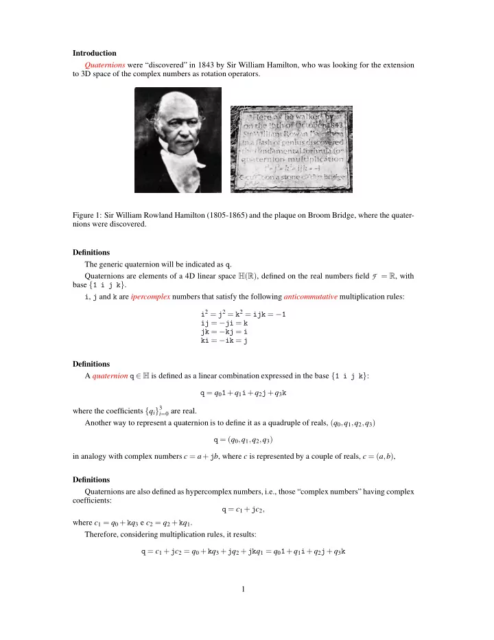
Introduction Quaternions were “discovered” in 1843 by Sir William Hamilton, who was looking for the extension to 3D space of the complex numbers as rotation operators. Figure 1: Sir William Rowland Hamilton (1805-1865) and the plaque on Broom Bridge, where the quater- nions were discovered. Definitions The generic quaternion will be indicated as q . Quaternions are elements of a 4D linear space H ( R ) , defined on the real numbers field F = R , with base { 1 i j k } . i , j and k are ipercomplex numbers that satisfy the following anticommutative multiplication rules: i 2 = j 2 = k 2 = ijk = − 1 ij = − ji = k jk = − kj = i ki = − ik = j Definitions A quaternion q ∈ H is defined as a linear combination expressed in the base { 1 i j k } : q = q 0 1 + q 1 i + q 2 j + q 3 k where the coefficients { q i } 3 i = 0 are real. Another way to represent a quaternion is to define it as a quadruple of reals, ( q 0 , q 1 , q 2 , q 3 ) q = ( q 0 , q 1 , q 2 , q 3 ) in analogy with complex numbers c = a + j b , where c is represented by a couple of reals, c = ( a , b ) , Definitions Quaternions are also defined as hypercomplex numbers, i.e., those “complex numbers” having complex coefficients: q = c 1 + j c 2 , where c 1 = q 0 + k q 3 e c 2 = q 2 + k q 1 . Therefore, considering multiplication rules, it results: q = c 1 + j c 2 = q 0 + k q 3 + j q 2 + jk q 1 = q 0 1 + q 1 i + q 2 j + q 3 k 1

Definitions In analogy with complex numbers that are the sum of a real part and an imaginary part, quaternions are the sum of a real part and a vectorial part. The real part q r is defined as q r = q 0 , and the vectorial part q v is defined as q v = q 1 i + q 2 j + q 3 k . We write q = ( q r , q v ) or q = q r + q v ; note that the vectorial part is not “transposed” since the conven- tional definition for the vectorial part of a quaternion assumes a row representation. Using the convention that defines vectors as “column” vectors, we can write q = ( q r , q T v ) . Definitions Quaternions are general mathematical objects, that include real numbers r = ( r , 0 , 0 , 0 ) , r ∈ R complex numbers a + i b = ( a , b , 0 , 0 ) , a , b ∈ R real vectors in R 3 (with some caution, since not all vectorial parts represents vectors) v = ( 0 , v 1 , v 2 , v 3 ) , v i ∈ R . k } are to be understood as unit vectors { i j k } forming an orthonor- In this last case, elements { i j mal base in a cartesian right-handed reference frame. Definitions Multiplication rules between elements i , j , k have the same properties of the cross product between unit vectors i , j , k : i × j = k ij = k ⇔ j × i = − k ji = − k ⇔ etc. In the following we will use all the possible alternative notations to indicate quaternions q = q 0 1 + q 1 i + q 2 j + q 3 k = ( q r , q v ) = q r + q v = ( q 0 , q 1 , q 2 , q 3 ) i.e., a) a hypercomplex number; b) the sum of a real part and a vectorial part; c) a quadruple of reals. Definitions An alternative way to write a quaternion is the following q = q 0 1 + q 1 i + q 2 j + q 3 k where now i i � � � � � � � � 1 0 0 0 1 0 1 = ; i = ; j = ; k = ; − i i 0 1 0 − 1 0 0 and i 2 = − 1. Hence every matrix is of the form c d � � ; − d ∗ c ∗ These matrices are called Cayley matrices [see Rotations - Pauli spin matrices ]. 2

Quaternions algebra Given a quaternion q = q 0 1 + q 1 i + q 2 j + q 3 k = q r + q v = ( q 0 , q 1 , q 2 , q 3 ) , the following properties hold: • a null or zero 0 quaternion exists 0 = 0 1 + 0 i + 0 j + 0 k = ( 0 , 0 ) = 0 + 0 = ( 0 , 0 , 0 , 0 ) • a conjugate quaternion q ∗ exists, having the same real part and the opposite vectorial part: q ∗ = q 0 − ( q 1 i + q 2 j + q 3 k ) = ( q r , − q v ) = q r − q v = ( q 0 , − q 1 , − q 2 , − q 3 ) Conjugate quaternions satisfy ( q ∗ ) ∗ = q Quaternions algebra • a non-negative function, called quaternion norm exists � q � , defined as 3 ∑ � q � 2 = qq ∗ = q ∗ q = q 2 ℓ = q 2 0 + q T v q v ℓ = 0 A quaternion with unit norm � q � = 1 is called unit quaternion . Quaternion q and its conjugate q ∗ have the same norm � q � = � q ∗ � The quaternion q v = 0 1 + q 1 i + q 2 j + q 3 k = ( 0 , q v ) = 0 + q v = ( 0 , q 1 , q 2 , q 3 ) , that has a zero real part is called pure quaternion or vector . The conjugate of a pure quaternion q v is the opposite of the original pure quaternion q ∗ v = − q v Quaternions algebra Given two quaternions h = h 0 1 + h 1 i + h 2 j + h 3 k = ( h r , h v ) = h r + h v = ( h 0 , h 1 , h 2 , h 3 ) and g = g 0 1 + g 1 i + g 2 j + g 3 k = ( g r , g v ) = g r + g v = ( g 0 , g 1 , g 2 , g 3 ) the following operations are defined Sum h + g Sum or addition ( h 0 + g 0 ) 1 + ( h 1 + g 1 ) i + ( h 2 + g 2 ) j + ( h 3 + g 3 ) k h + g = (( h r + g r ) , ( h v + g v )) = ( h r + g r )+ ( h v + g v ) = ( h 0 + g 0 , h 1 + g 1 , h 2 + g 2 , h 3 + g 3 ) = Difference Difference or subtraction ( h 0 − g 0 ) 1 + ( h 1 − g 1 ) i + ( h 2 − g 2 ) j + ( h 3 − g 3 ) k h − g = (( h r − g r ) , ( h v − g v )) = ( h r − g r )+ ( h v − g v ) = ( h 0 − g 0 , h 1 − g 1 , h 2 − g 2 , h 3 − g 3 ) = 3

Product Product ( h 0 g 0 − h 1 g 1 − h 2 g 2 − h 3 g 3 ) 1 + = hg ( h 1 g 0 + h 0 g 1 − h 3 g 2 + h 2 g 3 ) i + ( h 2 g 0 + h 3 g 1 + h 0 g 2 − h 1 g 3 ) j + ( h 3 g 0 − h 2 g 1 + h 1 g 2 + h 0 g 3 ) k ( h r g r − h v · g v , h r g v + g r h v + h v × g v ) = where h v · g v is the scalar product h v · g v = ∑ h vi g vi = h T v g v = g T v h v i defined in R n , and h v × g v is the cross product (defined only in R 3 ) � h 2 g 3 − h 3 g 2 � h v × g v = h 3 g 1 − h 1 g 3 = S ( h v ) g v h 1 g 2 − h 2 g 1 Product The quaternion product is anti-commutative, since, being g v × h v = − h v × g v it follows gh = ( h r g r − h v · g v , h r g v + g r h v − h v × g v ) � = hg ; Notice that the real part remains the same, while the vectorial part changes. Product commutes only if h v × g v = 0 , i.e., when the vectorial parts are parallel. The conjugate of a quaternion product satisfies ( gh ) ∗ = h ∗ g ∗ . The product norm satisfies � hg � = � h �� g � . Product properties • associative ( gh ) p = g ( hp ) • multiplication by the unit scalar 1q = q1 = ( 1 , 0 )( q r , q v ) = ( 1 q r , 1 q v ) = ( q r , q v ) • multiplication by the real λ λ q = ( λ , 0 )( q r , q v ) = ( λ q r , λ q v ) • bilinearity, with real λ 1 , λ 2 g ( λ 1 h 1 + λ 2 h 2 ) λ 1 gh 1 + λ 2 gh 2 = ( λ 1 g 1 + λ 2 g 2 ) h λ 1 g 1 h + λ 2 g 2 h = 4

Product Alternative forms Quaternion product may be written as matrix product forms: h 0 − h 1 − h 2 − h 3 g 0 g 0       h 1 h 0 − h 3 h 2 g 1 g 1 � h 0 − h T � v hg =  =       h 2 h 3 h 0 − h 1 g 2 g 2 h v h 0 I + S ( h v )      h 3 − h 2 h 1 h 0 g 3 g 3 = F L ( h ) g or g 0 − g 1 − g 2 − g 3 h 0 h 0       g 1 g 0 g 3 − g 2 h 1 h 1 � g 0 − g T � v hg =  =       g 2 − g 3 g 0 g 1 h 2 h 2 g v g 0 I − S ( g v )      g 3 g 2 − g 1 g 0 h 3 h 3 = F R ( g ) h Quotient Since the quaternion product is anti-commutative we must distinguish between the left and the right quotient or division. Given two quaternions h e p , we define the left quotient of p by h the quaternion q ℓ that satisfies hq ℓ = p while we define the right quotient of p by h the quaternion q r that satisfies q r h = p Hence h ∗ q r = p h ∗ q ℓ = � h � 2 p ; � h � 2 Inverse and the left inverse q − 1 Given a quaternion q , in principle one must define the right q − 1 as r ℓ qq − 1 q − 1 = 1 = ( 1 , 0 , 0 , 0 ) ; r q = 1 = ( 1 , 0 , 0 , 0 ) ℓ Since qq ∗ = q ∗ q = � q � 2 = � q �� q ∗ � , one can write q ∗ q ∗ q q � q ∗ � = � q � = 1 = ( 1 , 0 , 0 , 0 ) � q ∗ � � q � It follows that right inverse and left inverse are equal q ∗ c ∗ = q − 1 = c − 1 = q − 1 = q − 1 similar to r ℓ � q � 2 � c � 2 Inverse For a unit quaternion u , � u � = 1, inverse and conjugate coincide u − 1 = u ∗ , � u � = 1 and for a pure unit quaternion q = ( 0 , q v ) , � q � = 1, i.e., a unit vector q − 1 = q ∗ v = − q v . v Inverse satisfies ( q − 1 ) − 1 = q ; ( pq ) − 1 = q − 1 p − 1 5