Definition of impulse response model g ( n ) : { ( n ) } Time - - PowerPoint PPT Presentation

1.

Impulse Response Models for LTI Systems

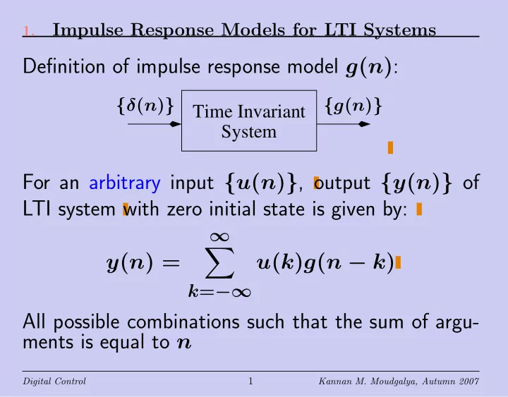
Definition of impulse response model g(n):

Time Invariant System

{g(n)} {δ(n)}

For an arbitrary input {u(n)}, output {y(n)} of LTI system with zero initial state is given by: y(n) =

∞

• k=−∞

u(k)g(n − k) All possible combinations such that the sum of argu- ments is equal to n

Digital Control

1

Kannan M. Moudgalya, Autumn 2007

2.

Importance of Impulse Response Models

• Impulse response has all information about LTI sys-

tem

• Given impulse response, can determine output due

to any arbitrary input

Digital Control

2

Kannan M. Moudgalya, Autumn 2007

3.

Step Response, Relation with Impulse Response

The unit step response of an LTI system at zero ini- tial state {s(n)} is the output when {u(n)} = {1(n)}: s(n) =

∞

• k=−∞

1(k)g(n − k) Apply the meaning of 1(k): =

∞

• k=0

g(n − k)

• This shows that the step response is the sum of

impulse response.

Digital Control

3

Kannan M. Moudgalya, Autumn 2007

4.

Relation between Step and Impulse Responses

• We can also get impulse response from step re-

sponse. δ(n) = 1(n) − 1(n − 1) Using linearity and time invariance properties, g(n) = s(n) − s(n − 1)

Digital Control

4

Kannan M. Moudgalya, Autumn 2007

5.

Causality of LTI Systems

• If output depends only on past inputs, called causal
• If output depends on future inputs, not causal
• For LTI causal systems, g(n) = 0 for n < 0

– Initial state is zero – No input until n = 0 - impulse input – So, impulse response can begin only from n = 0

• Signal {u(n)} is causal if u(k) = 0 for k < 0

Digital Control

5

Kannan M. Moudgalya, Autumn 2007

6.

Output of Causal Systems to Causal Signals

• Impulse response g(n), input u(n) are causal:

y(n) =

∞

• k=−∞

u(k)g(n − k) =

∞

• k=0

u(k)g(n − k) (u(k) = 0 ∀k < 0) =

n

• k=0

u(k)g(n − k) (g(k) = 0 ∀k < 0)

Digital Control

6

Kannan M. Moudgalya, Autumn 2007

7.

Convolution Theorems

Convolution is Commutative: u(n) ∗ g(n) = g(n) ∗ u(n) Convolution is Associative:

u(n) ∗ (g1(n) ∗ g2(n)) = (u(n) ∗ g1(n)) ∗ g2(n)

Convolution Distributes over Addition: u(n) ∗ (g1(n) + g2(n)) = u(n) ∗ g1(n) + u(n)

g1(n) + g2(n) u(n) y1(n) y2(n)

+

u(n) g2(n) g1(n)

Digital Control

7

Kannan M. Moudgalya, Autumn 2007

8.

External (BIBO) Stability of LTI Systems

If every Bounded Input produces Bounded Output,

• system is externally stable
• equivalently, system is BIBO stable

∞

• n=−∞

|g(n)| < ∞ ⇔ BIBO Stability

• Don’t care about what unbounded input does...

Digital Control

8

Kannan M. Moudgalya, Autumn 2007

9.

Recall convolution example

{y(n)} =

∞

• k=−∞

u(k){g(n − k)} {g(n)} = {1, 2, 3}, {u(n)} = {4, 5, 6} g, u start at n = 0. They are zero for n < 0. y(0) = u(0)g(0) = 4 y(1) = u(0)g(1) + u(1)g(0) = 13 y(2) = u(0)g(2) + u(1)g(1) + u(2)g(0) = 28 y(3) = u(1)g(2) + u(2)g(1) = 27 y(4) = u(2)g(2) = 18 All other terms that don’t appear above are zero.

Digital Control

9

Kannan M. Moudgalya, Autumn 2007

10.

Polynomial Calculation ≡ Convolution

Also carryout multiplication:

(u(0)+u(1)z−1+u(2)z−2)×(g(0)+g(1)z−1+g(2)z−2) =

u(0)g(0) + (u(0)g(1) + u(1)g(0))z−1 + (u(0)g(2) + u(1)g(1) + u(2)g(0))z−2 + (u(1)g(2) + u(2)g(1))z−3 +

• z a position marker - coeff. of z−i at ith instant
• u(0)+u(1)z−1+u(2)z−2 - a way of represent-

ing a sequence with three terms: {u(0), u(1), u(2)}

• Even if large no. of terms, can get compact form

Digital Control

10

Kannan M. Moudgalya, Autumn 2007

11.

Definition of Z-transform

Z-transform of a sequence {u(n)}, denoted by U(z), is defined as: U(z) =

∞

• n=−∞

u(n)z−n where z is such that there is absolute convergence. That is, z should be chosen so as to satisfy

∞

• n=−∞

|u(n)z−n| < ∞

Digital Control

11

Kannan M. Moudgalya, Autumn 2007

12.

Important properties of transfer functions

Given a causal, BIBO stable system with impulse re- sponse g(n)

• Z-transform of g(n), namely G(z), will have poles

inside unit circle g(n) is a causal sequence

• G(z) = N(z)

D(z) with

– N(z) is a polynomial of degree n – D(Z) is a polynomial of degree m

• n ≤ m

Digital Control

12

Kannan M. Moudgalya, Autumn 2007

13.

Z-transform Theorems - Linearity

Given the following Z-transform pairs, u1(n) ↔ U1(z), u2(n) ↔ U2(z), the following relation, with arbitrary α, β, holds:

Z [α{u1(n)} + β{u2(n)}] = αU1(z) + βU2(z)

Digital Control

13

Kannan M. Moudgalya, Autumn 2007

14.

Example 1 - Linearity

Find the Z-transform of u1(n) = δ(n) − 3δ(n − 2):

U1(z) =

∞

• n=−∞

δ(n)z−n − 3

∞

• n=−∞

δ(n − 2)z−n = 1 − 3z−2 ∀z−1 finite

Digital Control

14

Kannan M. Moudgalya, Autumn 2007

15.

Z-transform - Shifting

Z [u(n + d)] =

∞

• n=−∞

u(n + d)z−n = zd

∞

• n=−∞

u(n + d)z−(n+d) = zdU(z)

Digital Control

15

Kannan M. Moudgalya, Autumn 2007

16.

Z-transform - Shifting

Example: If {u(n)} ↔ U(z), then {u(n + 3)} ↔ z3U(z) {u(n − 2)} ↔ z−2U(z)

Digital Control

16

Kannan M. Moudgalya, Autumn 2007

17.

Initial value, theorem for causal signals

lim

z→∞ U(z) = u(0)

Digital Control

17

Kannan M. Moudgalya, Autumn 2007

18.

Final value theorem for causal signals

• Under the conditions

– U(z) converges for all |z| > 1, – if all poles of U(z)(1 − z−1) are inside unit circle, lim

k→∞ u(k) = lim z→1(1 − z−1)U(z)

Digital Control

18

Kannan M. Moudgalya, Autumn 2007

19.

Examples for Final Value Theorem

Using the final value theorem, find the steady state value of (0.5n − 0.5)1(n) and verify. (0.5n − 0.5)1(n) ↔ z z − 0.5 − 0.5z z − 1 |z| > 1 lim

n→∞ LHS = −0.5

lim

z→1(z − 1)RHS = − lim z→1

0.5z z − 1(z − 1) = −0.5

Digital Control

19

Kannan M. Moudgalya, Autumn 2007

20.

Examples for Final Value Theorem

Is it possible to use the final value theorem on 2n1(n)? 2n1(n) ↔ z z − 2 |z| > 2

• Since RHS is valid only for |z| > 2, the theorem

cannot even be applied.

• In the LHS also, there is a pole outside the unit cir-

cle thereby violating the conditions of the theorem.

Digital Control

20

Kannan M. Moudgalya, Autumn 2007

21.

Z-transform of Convolution

If u(n) ↔ U(z) g(n) ↔ G(z) then, g(n) ∗ u(n) ↔ G(z)U(z) Recall the motivation slide for Z-transform.

Digital Control

21

Kannan M. Moudgalya, Autumn 2007

22.

Z-transform of Discrete State Space Systems

x(n + 1) = Ax(n) + Bu(n) x(0) = x0 Invalid for n = −1: x(0) = Ax(−1) + Bu(−1) = 0 = x0 The fact that it is not valid for n < 0 is not explicitly

• stated. But if we write it as

x(n + 1) = Ax(n) + Bu(n) + δ(n + 1)x0 and assume initial rest, all variables are zero until n = 0, problem is solved.

Digital Control

22

Kannan M. Moudgalya, Autumn 2007

23.

Z-transform of Discrete State Space Systems Z-transform of x(n + 1) = Ax(n) + Bu(n) + δ(n + 1)x0 gives zX(z) = AX(z) + BU(z) + x0z (zI − A)X(z) = BU(z) + x0z X(z) = (zI − A)−1BU(z) + z(zI − A)−1x0 Z-transform of y(n) = Cx(n) + Du(n) is Y (z) = CX(z) + DU(z) = C(zI − A)−1BU(z) + DU(z) + C(zI − A)−1zx(0) = [C(zI − A)−1B + D]U(z) + C(zI − A)−1zx(0)

Digital Control

23

Kannan M. Moudgalya, Autumn 2007

24.

Finding Transfer Function - an Example Find the transfer function of A =

• 1

0.19801 0.9802

• ,

B =

• 0.02

0.001987

• C =
• 0 1
• ,

D = 0, G = c(zI − A)−1B =

• 0 1

z − 1 −0.19801 z − 0.9802 −1 0.02 0.001987

• =
• 0 1
• (z − 1)(z − 0.9802)

z − 0.9802 0.19801 z − 1 0.02 0.001987

• Digital Control

24

Kannan M. Moudgalya, Autumn 2007

25.

Finding Transfer Function - an Example G =

• 0 1
• (z − 1)(z − 0.9802)

z − 0.9802 0.19801 z − 1 0.02 0.001987

• =
• 0.19801 z − 1
• (z − 1)(z − 0.9802)
• 0.02

0.001987

• = 0.001987z + 0.0019732

(z − 1)(z − 0.9802) = 0.001987 z + 0.9931 (z − 1)(z − 0.9802)

Digital Control

25

Kannan M. Moudgalya, Autumn 2007

26.

Finding Transfer Function - an Example

1

/ / U p d a t e d ( 1 8 − 7 − 0 7 )

2

/ / 4 . 4

3 4 F = [0

0; 1 −0.1]; G = [ 0 . 1 ; 0 ] ;

5 C = [0

1 ] ; dt = 0 . 2 ;

6 sys = syslin ( ’ c ’ ,F ,G,C) ; 7 sysd = dscr ( sys , dt ) ; 8 H = ss2tf ( sysd ) ;

Digital Control

26

Kannan M. Moudgalya, Autumn 2007