
SLIDE 1
1
Chapter 3 Convolution Representation Chapter 3 Convolution Representation
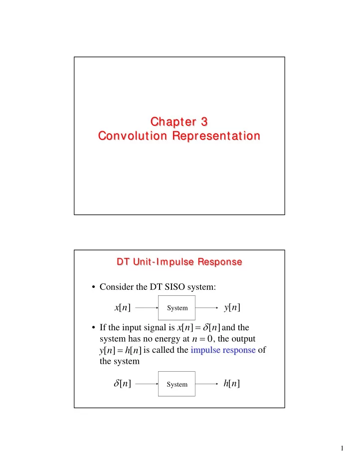
- Consider the DT SISO system:
- If the input signal is and the
system has no energy at , the output is called the impulse response impulse response of the system DT Unit-Impulse Response DT Unit-Impulse Response
[ ] y n [ ] x n [ ] h n [ ] n δ [ ] [ ] x n n δ = [ ] [ ] y n h n =
System System