[PDF] - Data Mining Ian H. Witten The problem Data Mining with Weka PDF Document

SLIDE 1

Data Mining

Ian H. Witten

Data Mining with Weka

Ian H. Witten Computer Science Department Waikato University New Zealand http://www.cs.waikato.ac.nz/~ihw http://www.cs.waikato.ac.nz/ml/weka

The problem

Classification (“supervised”) Given  A set of classified examples Produce  A way of classifying new examples Instances: described by fixed set of features Classes: discrete or continuous Interested in: Results? (classifying new instances) Model? (how the decision is made) “instances” “attributes” “classification” “regression” Association rules Look for rules that relate features to other features Clustering (“unsupervised”) There are no classes

Simplicity first!

 Simple algorithms often work very well!  There are many kinds of simple structure, eg:

 One attribute does all the work  All attributes contribute equally and independently  A decision tree involving tests on a few attributes  Rules that assign instances to classes  Distance in instance space from a few class “prototypes”  Result depends on a linear combination of attributes

 Success of method depends on the domain

Agenda

 A very simple strategy

 Overfitting, evaluation

 Statistical modeling

 Bayes rule

 Constructing decision trees  Constructing rules

 + Association rules

 Linear models

 Regression, perceptrons, neural nets, SVMs, model trees

 Instance-based learning and clustering

 Hierarchical, probabilistic clustering

 Engineering the input and output

 Attribute selection, data transformations, PCA  Bagging, boosting, stacking, co-training

One attribute does all the work

 Learn a 1-level decision tree

 i.e., rules that all test one particular attribute

 Basic version

 One branch for each value  Each branch assigns most frequent class  Error rate: proportion of instances that don’t belong to the majority class of their corresponding branch  Choose attribute with smallest error rate

For each attribute, For each value of the attribute, make a rule as follows: count how often each class appears find the most frequent class make the rule assign that class to this attribute-value Calculate the error rate of this attribute’s rules Choose the attribute with the smallest error rate

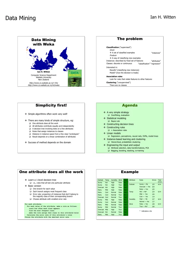
Example

3/6 True → No* 5/14 2/8 False → Yes Wind 1/7 Normal → Yes 4/14 3/7 High → No Humidity 5/14 4/14 Total errors 1/4 Cool → Yes 2/6 Mild → Yes 2/4 Hot → No* Temp 2/5 Rainy → Yes 0/4 Overcast → Yes 2/5 Sunny → No Outlook Errors Rules Attribute * indicates a tie No True High Mild Rainy Yes False Normal Hot Overcast Yes True High Mild Overcast Yes True Normal Mild Sunny Yes False Normal Mild Rainy Yes False Normal Cool Sunny No False High Mild Sunny Yes True Normal Cool Overcast No True Normal Cool Rainy Yes False Normal Cool Rainy Yes False High Mild Rainy Yes False High Hot Overcast No True High Hot Sunny No False High Hot Sunny Play Wind Humidity Temp Outlook No True High Mild Rainy Yes False Normal Hot Overcast Yes True High Mild Overcast Yes True Normal Mild Sunny Yes False Normal Mild Rainy Yes False Normal Cool Sunny No False High Mild Sunny Yes True Normal Cool Overcast No True Normal Cool Rainy Yes False Normal Cool Rainy Yes False High Mild Rainy Yes False High Hot Overcast No True High Hot Sunny No False High Hot Sunny Play Wind Humidity Temp Outlook

SLIDE 2

Data Mining

Ian H. Witten

Complications: Missing values

 Omit instances where the attribute value is missing  Treat “missing” as a separate possible value “Missing” means what?  Unknown?  Unrecorded?  Irrelevant? Is there significance in the fact that a value is missing?  Nominal vs numeric values for attributes

Complications: Overfitting

… … … … … Yes False 80 75 Rainy Yes False 86 83 Overcast No True 90 80 Sunny No False 85 85 Sunny Play Wind Humidity Temp Outlook 0/14 Total errors … … 0/1 75 → Yes 0/1 83 → Yes 0/1 80 → No 0/1 85 → No Temp Errors Rules Attribute

 Memorization vs generalization  Do not evaluate rules on the training data  Here, independent test data shows poor performance  To fix, use

 Training data — to form rules  Validation data — to decide on best rule  Test data — to determine system performance

 Evaluate on training set? — NO!  Independent test set  Cross-validation  Stratified cross-validation  Stratified 10-fold cross-validation, repeated 10 times  Leave-one-out  The “Bootstrap”

Evaluating the result

 This incredibly simple method was described in a 1993 paper

 An experimental evaluation on 16 datasets  Used cross-validation so that results were representative of performance on new data  Simple rules often outperformed far more complex methods

 Simplicity first pays off!

“Very Simple Classification Rules Perform Well on Most Commonly Used Datasets” Robert C. Holte, Computer Science Department, University of Ottawa

One attribute does all the work Agenda

 A very simple strategy

 Overfitting, evaluation

 Statistical modeling

 Bayes rule

 Constructing decision trees  Constructing rules

 + Association rules

 Linear models

 Regression, perceptrons, neural nets, SVMs, model trees

 Instance-based learning and clustering

 Hierarchical, probabilistic clustering

 Engineering the input and output

 Attribute selection, data transformations, PCA  Bagging, boosting, stacking, co-training

Statistical modeling

 Opposite strategy: use all the attributes  Two assumptions: Attributes are

 equally important a priori  statistically independent (given the class value)

I.e., knowing the value of one attribute says nothing about the value of another (if the class is known)

 Independence assumption is never correct!  But … often works well in practice One attribute does all the work?

SLIDE 3

Data Mining

Ian H. Witten

 Probability of event H given evidence E  A priori probability of H

 Probability of event before evidence is seen

 A posteriori probability of H

 Probability of event after evidence is seen

Bayes’s rule

] Pr[ ] Pr[ ] | Pr[ ] | Pr[ E H H E E H = ] | Pr[ E H ] Pr[H

Thomas Bayes British mathematician and Presbyterian minister Born 1702 Died 1761

Pr[H | E] = Pr[E1 | H]Pr[E1 | H]...Pr[En | H]Pr[H] Pr[E]

 “Naïve” assumption:

 Evidence splits into parts that are independent instance class

Weather data: probabilities

5/14 5 No 9/14 9 Yes Play 3/5 2/5 3 2 No 3/9 6/9 3 6 Yes True False True False Wind 1/5 4/5 1 4 No Yes No Yes No Yes 6/9 3/9 6 3 Normal High Normal High Humidity 1/5 2/5 2/5 1 2 2 3/9 4/9 2/9 3 4 2 Cool 2/5 3/9 Rainy Mild Hot Cool Mild Hot Temperature 0/5 4/9 Overcast 3/5 2/9 Sunny 2 3 Rainy 4 Overcast 3 2 Sunny Outlook

No True High Mild Rainy Yes False Normal Hot Overcast Yes True High Mild Overcast Yes True Normal Mild Sunny Yes False Normal Mild Rainy Yes False Normal Cool Sunny No False High Mild Sunny Yes True Normal Cool Overcast No True Normal Cool Rainy Yes False Normal Cool Rainy Yes False High Mild Rainy Yes False High Hot Overcast No True High Hot Sunny No False High Hot Sunny Play Wind Humidity Temp Outlook

5/14 5 No 9/14 9 Yes Play 3/5 2/5 3 2 No 3/9 6/9 3 6 Yes True False True False Wind 1/5 4/5 1 4 No Yes No Yes No Yes 6/9 3/9 6 3 Normal High Normal High Humidity 1/5 2/5 2/5 1 2 2 3/9 4/9 2/9 3 4 2 Cool 2/5 3/9 Rainy Mild Hot Cool Mild Hot Temperature 0/5 4/9 Overcast 3/5 2/9 Sunny 2 3 Rainy 4 Overcast 3 2 Sunny Outlook ? True High Cool Sunny Play Wind Humidity Temp. Outlook

 A new day:

Likelihood of the two classes For “yes” = 2/9 × 3/9 × 3/9 × 3/9 × 9/14 = 0.0053 For “no” = 3/5 × 1/5 × 4/5 × 3/5 × 5/14 = 0.0206 Conversion into a probability by normalization: P(“yes”) = 0.0053 / (0.0053 + 0.0206) = 0.205 P(“no”) = 0.0206 / (0.0053 + 0.0206) = 0.795

Weather data: probabilities

? True High Cool Sunny Play Wind Humidity Temp. Outlook

] Pr[

14 9 9 3 9 3 9 3 9 2

E ! ! ! ! =

Weather data: probabilities

 Training: do not include instance in frequency count for attribute value-class combination  Classification: omit attribute from calculation  Example:

Missing values

? True High Cool ? Play Wind Humidity Temp. Outlook Likelihood of “yes” = 3/9 × 3/9 × 3/9 × 9/14 = 0.0238 Likelihood of “no” = 1/5 × 4/5 × 3/5 × 5/14 = 0.0343 P(“yes”) = 0.0238 / (0.0238 + 0.0343) = 41% P(“no”) = 0.0343 / (0.0238 + 0.0343) = 59%

Complications

Zero frequencies

 An attribute value doesn’t occur with every class

 Probability will be zero!

] | Pr[ = = yes High Humidity

Numeric attributes

 Often assume attributes have a Gaussian distribution (given the class)  Its probability density function is defined by two parameters:

 Sample mean  Standard deviation

 The density function is

!

=

n i i

x n

1

1 µ

!

=

" " =

n i i

x n

1 2

) ( 1 1 µ #

2 2

2 ) (

2 1 ) (

! µ

! "

# #

=

x

e x f Carl Friedrich Gauss

German mathematician and scientist “The prince of mathematicians” Born 1777 Died 1855

SLIDE 4

Data Mining

Ian H. Witten

Numeric attributes

 Often assume attributes have a Gaussian distribution (given the class)  Its probability density function is defined by two parameters:

 Sample mean  Standard deviation

 The density function is

!

=

n i i

x n

1

1 µ

!

=

" " =

n i i

x n

1 2

) ( 1 1 µ #

2 2

2 ) (

2 1 ) (

! µ

! "

# #

=

x

e x f

 A new day:

? true 90 66 Sunny Play Wind Humidity Temp. Outlook

Likelihood of “yes” = 2/9 × 0.0340 × 0.0221 × 3/9 × 9/14 = 0.000036 Likelihood of “no” = 3/5 × 0.0291 × 0.0380 × 3/5 × 5/14 = 0.000136 P(“yes”) = 0.000036 / (0.000036 + 0. 000136) = 20.9% P(“no”) = 0.000136 / (0.000036 + 0. 000136) = 79.1%

“Naïve” statistical model

Naïve = assume attributes are independent  Naïve Bayes works surprisingly well

 even if independence assumption is clearly violated

 Why?

 Because classification doesn’t require accurate probability estimates  so long as the greatest probability is assigned to the correct class

 But: adding redundant attributes causes problems

 e.g. identical attributes

 And: numeric attributes may not be normally distributed

 → kernel density estimators

Agenda

 A very simple strategy

 Overfitting, evaluation

 Statistical modeling

 Bayes rule

 Constructing decision trees  Constructing rules

 + Association rules

 Linear models

 Regression, perceptrons, neural nets, SVMs, model trees

 Instance-based learning and clustering

 Hierarchical, probabilistic clustering

 Engineering the input and output

 Attribute selection, data transformations, PCA  Bagging, boosting, stacking, co-training

Constructing decision trees

 Strategy: top down Recursive divide-and-conquer fashion

 First: select attribute for root node Create branch for each possible attribute value  Then: split instances into subsets One for each branch extending from the node  Finally: repeat recursively for each branch, using only instances that reach the branch

 Stop if all instances have the same class

Which attribute to select? Which is the best attribute?

 Criterion: want to get the smallest tree  Heuristic

 choose the attribute that produces the “purest” nodes  I.e. the greatest information gain

 Information theory: measure information in bits  Information gain

 Amount of information gained by knowing the value of the attribute  Entropy of distribution before the split – entropy of distribution after it entropy(p1, p2,..., pn) = "p1logp1 " p2logp2..." pnlogpn

Claude Shannon American mathematician and scientist “The father of information theory” Born 1916 Died 2001

SLIDE 5

Data Mining

Ian H. Witten

Which attribute to select?

0.247 bits 0.152 bits 0.048 bits 0.029 bits

Continuing to split

gain(temperature ) = 0.571 bits gain(humidity ) = 0.971 bits gain(windy ) = 0.020 bits

Complications

 Highly-branching attributes

 Extreme case: ID code

n m l k j i h g f e d c b a ID code No True High Mild Rainy Yes False Normal Hot Overcast Yes True High Mild Overcast Yes True Normal Mild Sunny Yes False Normal Mild Rainy Yes False Normal Cool Sunny No False High Mild Sunny Yes True Normal Cool Overcast No True Normal Cool Rainy Yes False Normal Cool Rainy Yes False High Mild Rainy Yes False High Hot Overcast No True High Hot Sunny No False High Hot Sunny Play Wind Humidity Temp Outlook

Info gain is maximal (0.940 bits)

Complications

 Highly-branching attributes

 Extreme case: ID code

 Overfitting: need to prune

good good good bad {good,bad} Acceptability of contract half full ? none {none,half,full} Health plan contribution yes ? ? no {yes,no} Bereavement assistance full full ? none {none,half,full} Dental plan contribution yes ? ? no {yes,no} Long-term disability assistance avg gen gen avg {below-avg,avg,gen} Vacation 12 12 15 11 (Number of days) Statutory holidays ? ? ? yes {yes,no} Education allowance Shift-work supplement Standby pay Pension Working hours per week Cost of living adjustment Wage increase third year Wage increase second year Wage increase first year Duration Attribute 4 4% 5% ? Percentage ? ? 13% ? Percentage ? ? ? none {none,ret-allw, empl-cntr} 40 38 35 28 (Number of hours) none ? tcf none {none,tcf,tc} ? ? ? ? Percentage 4.0 4.4% 5% ? Percentage 4.5 4.3% 4% 2% Percentage 2 3 2 1 (Number of years) 40 … 3 2 1 Type

Complications

 Highly-branching attributes

 Extreme case: ID code

 Overfitting: need to prune

Complications

 Highly-branching attributes

 Extreme case: ID code

 Overfitting: need to prune

 Prepruning vs postpruning

 Missing values

 During training  During testing: “fractional instances”

 Numeric attributes

 Choose best “split point” for attribute  E.g. temp < 25

SLIDE 6

Data Mining

Ian H. Witten

 The most extensively studied method of machine learning used in data mining  Different criteria for attribute selection

 rarely make a large difference

 Different pruning methods

 mainly change the size of the pruned tree

 Univariate vs multivariate decision trees

 Single vs compound tests at the nodes

 C4.5 and CART

Constructing decision trees

Top-down induction of decision trees

Ross Quinlan Australian computer scientist University of Sydney

Agenda

 A very simple strategy

 Overfitting, evaluation

 Statistical modeling

 Bayes rule

 Constructing decision trees  Constructing rules

 + Association rules

 Linear models

 Regression, perceptrons, neural nets, SVMs, model trees

 Instance-based learning and clustering

 Hierarchical, probabilistic clustering

 Engineering the input and output

 Attribute selection, data transformations, PCA  Bagging, boosting, stacking, co-training

Constructing rules

 Convert (top-down) decision tree into a rule set

 Straightforward, but rule set overly complex  More effective conversions are not trivial

 Alternative: (bottom-up) covering method

 for each class in turn find rule set that covers all instances in it (excluding instances not in the class)

 Separate-and-conquer method

 First identify a useful rule  Then separate out all the instances it covers  Finally “conquer” the remaining instances

 Cf divide-and-conquer methods:

 No need to explore subset covered by rule any further

Generating a rule

y x a b b b b b b b b b b b b b b a a a a a

y a b b b b b b b b b b b b b b a a a a a x 1·2 y a b b b b b b b b b b b b b b a a a a a x 1·2 2·6

If x > 1.2 then class = a If x > 1.2 and y > 2.6 then class = a If true then class = a

 Possible rule set for class “b”:  Could add more rules, get “perfect” rule set

If x ≤ 1.2 then class = b If x > 1.2 and y ≤ 2.6 then class = b

 Corresponding decision tree: (produces exactly the same predictions)  Rule sets can be more perspicuous

 E.g. when decision trees contain replicated subtrees

 Also: in multiclass situations,

 covering algorithm concentrates on one class at a time  decision tree learner takes all classes into account

Rules vs. trees

If x ≤ 1.2 then class = b If x > 1.2 and y ≤ 2.6 then class = b

For each class C  Initialize E to the instance set  While E contains instances in class C

Create a rule R that predicts class C

(with empty left-hand side)

Until R is perfect

(or there are no more attributes to use)

For each attribute A not mentioned in R, and each

value v,  Consider adding the condition A = v to the left- hand side of R  Select A and v to maximize the accuracy p/t (break ties by choosing the condition with the largest p)

Add A = v to R
Remove the instances covered by R from E

Constructing rules

SLIDE 7

Data Mining

Ian H. Witten

More about rules

 Rules are order-dependent

 Two rules might assign different classes to an instance

 Work through the classes in turn

 generating rules for that class

 For each class a “decision list” is generated

 Subsequent rules are designed for instances that are not covered by previous rules  But: order doesn’t matter because all rules predict the same class

 Problems: overlapping rules  For better rules: globalization optimization

Association rules

 … can predict any attribute and combinations of attributes  … are not intended to be used together as a set

 Problem: immense number of possible associations

 Output needs to be restricted to show only the most predictive associations

 Define

 Support: number of instances predicted correctly  Confidence: correct predictions as % of instances covered

 Examples  Specify minimum support and confidence

 e.g. 58 rules with support ≥ 2 and confidence ≥ 95%

If temperature = cool then humidity = normal

No True High Mild Rainy Yes False Normal Hot Overcast Yes True High Mild Overcast Yes True Normal Mild Sunny Yes False Normal Mild Rainy Yes False Normal Cool Sunny No False High Mild Sunny Yes True Normal Cool Overcast No True Normal Cool Rainy Yes False Normal Cool Rainy Yes False High Mild Rainy Yes False High Hot Overcast No True High Hot Sunny No False High Hot Sunny Play Wind Humidity Temp Outlook

If Wind = false and play = no then outlook = sunny and humidity = high Support = 4, confidence = 100% Support = 2, confidence = 100%

Constructing association rules

 To find association rules:

 Use separate-and-conquer  Treat every possible combination of attribute values as a separate class

 Two problems:

 Computational complexity  Huge number of rules (which would need pruning on the basis of support and confidence)

 But: we can look for high support rules directly!

 Generate frequent “item sets”  From them, generate and test possible rules

Temperature = Cool, Humidity = Normal, Wind = False, Play = Yes (2) Temperature = Cool, Wind = False ⇒ Humidity = Normal, Play = Yes Temperature = Cool, Wind = False, Humidity = Normal ⇒ Play = Yes Temperature = Cool, Wind = False, Play = Yes ⇒ Humidity = Normal

(all have support 2, confidence = 100%)

Example association rules

 Rules with support ≥ 2 and confidence 100%: support=4

3 rules support=3 5 rules support=2 50 rules total 58

100% 2 ⇒ Humidity=High Outlook=Sunny Temperature=Hot 58 ... ... ... ... 100% 3 ⇒ Humidity=Normal Temperature=Cold Play=Yes 4 100% 4 ⇒ Play=Yes Outlook=Overcast 3 100% 4 ⇒ Humidity=Normal Temperature=Cool 2 100% 4 ⇒ Play=Yes Humidity=Normal Wind=False 1 Association rule Conf. Sup.

Association rules: discussion

 Market basket analysis: huge data sets  May not fit in main memory

 Different algorithms necessary  Minimize passes through the data

 Practical issue: generating a certain number of rules

 e.g. by incrementally reducing minimum support

 Confidence is not necessarily the best measure

 e.g. milk occurs in almost every supermarket transaction  Other measures have been devised (e.g. lift)

Buy beer ⇒ buy chips Day = Thursday, buy beer ⇒ buy diapers

Agenda

 A very simple strategy

 Overfitting, evaluation

 Statistical modeling

 Bayes rule

 Constructing decision trees  Constructing rules

 + Association rules

 Linear models

 Regression, perceptrons, neural nets, SVMs, model trees

 Instance-based learning and clustering

 Hierarchical, probabilistic clustering

 Engineering the input and output

 Attribute selection, data transformations, PCA  Bagging, boosting, stacking, co-training

SLIDE 8

Data Mining

Ian H. Witten

Linear models

 Standard technique: linear regression

 Works most naturally with numeric attributes  Outcome is linear combination of attributes

 Calculate weights from the training data  Predicted value for first training instance a(1)

k ka

w a w a w w x + + + + = ...

2 2 1 1

!

=

= + + + +

k j j j k k

a w a w a w a w a w

) 1 ( ) 1 ( ) 1 ( 2 2 ) 1 ( 1 1 ) 1 (

...  Choose weights to minimize squared error on the training data  Standard matrix problem

 Works if there are more instances than attributes (roughly speaking)

2 1 ) ( ) (

! !

= =

" " # $ % % & ' (

n i k j i j j i

a w x

“Regression” = predicting a numeric quantity

Classification by regression

 Method 1: Multi-response linear regression

 Training: perform a regression for each class

set output to 1 for training instances that belong to the class,

0 for those that don’t

 Prediction: predict class that produces the largest output

 Method 2: Pairwise linear regression

 Find a regression function for every pair of classes, using only instances from these two classes

Assign output of +1 to one class, –1 to the other

 Prediction: use voting

Class that receives most votes is predicted
Alternative: “don’t know” if there is no agreement

 Method 3: Logistic regression

 Alternative to linear regression, designed for classification  Tries to estimate the class probabilities directly

Advanced linear models

 Linear model inappropriate if data exhibits non- linear dependencies  But: can serve as building blocks for more complex schemes  Support vector machine

 Resilient to overfitting  Learn a particular kind of decision boundary

 Multilayer perceptron

 Network of linear classifiers can approximate any target concept  An example of an artificial neural network

 Model tree

 Decision tree with linear model at the nodes

Support vector machine

The support vectors define the maximum margin hyperplane All other instances can be deleted without changing it!

maximum margin hyperplane support vectors

Multilayer perceptron

 Network of linear classifiers

 Input layer, hidden layer(s), and output layer

 Parameters are found by backpropagation  Minimize error using “gradient descent”  Can get excellent results  Involves experimentation input

utput

Trees for numeric prediction

 Regression tree

 each leaf predicts a numeric quantity  Predict the average value of training instances at the leaf

 Model tree

 each leaf has a linear regression models  Linear patches approximate continuous function

SLIDE 9

Data Mining

Ian H. Witten

Discussion of linear models

 Linear regression: well-founded mathematical technique  Can be used for classification in situations that are “linearly separable”  … but very susceptible to noise  Support vector machines yield excellent performance

 particularly in situations with many redundant attributes

 Multilayer perceptrons (“neural nets”) can work well

 but often require much experimentation

 Regression/model trees grew out of decision trees

 Regression trees were introduced in CART  Model trees were developed by Quinlan

Agenda

 A very simple strategy

 Overfitting, evaluation

 Statistical modeling

 Bayes rule

 Constructing decision trees  Constructing rules

 + Association rules

 Linear models

 Regression, perceptrons, neural nets, SVMs, model trees

 Instance-based learning and clustering

 Hierarchical, probabilistic clustering

 Engineering the input and output

 Attribute selection, data transformations, PCA  Bagging, boosting, stacking, co-training

Instance-based learning

 Search training set for instance that’s most like the new one

 The instances themselves represent the “knowledge”  Noise will be a problem

 Similarity function defines what’s “learned”

 Euclidean distance  Nominal attributes? Set to 1 if different, 0 if same  Weight the attributes?

 Lazy learning: do nothing until you have to  Methods:

 nearest-neighbor  k-nearest-neighbor

“Rote learning” = simplest form of learning

 Often very accurate  … but slow:

 scan entire training data to make each prediction?  sophisticated data structures can make this much faster

 Assumes all attributes are equally important

 Remedy: attribute selection or weights

 Remedies against noisy instances:

 Majority vote over the k nearest neighbors  Weight instances according to their prediction accuracy  Identify reliable “prototypes” for each class

 Statisticians have used k-NN since 1950s

 If n → ∞ and k/n → 0, error approaches minimum

Instance-based learning Clustering

 No target value to predict  Differences between models/algorithms:

 Exclusive vs. overlapping  Hierarchical vs. flat  Incremental vs. batch learning  Deterministic vs. probabilistic

 Evaluation?

 Usually by inspection  Clusters-to-classes evaluation?  Probabilistic density estimation can be evaluated on test data

Unsupervised vs supervised learning (classification)

Hierarchical clustering

 Bottom up

 Start with single-instance clusters  At each step, join the two closest clusters  How to define the distance between clusters?

Distance between the two closest instances?
Distance between the means

 Top down

 Start with one universal cluster  Find two clusters  Proceed recursively

n each subset

SLIDE 10

Data Mining

Ian H. Witten

To cluster data into k groups (k is predefined)

1. Choose k cluster centers (“seeds”)

 e.g. at random

2. Assign instances to clusters

 based on distance to cluster centroids

3. Compute centroids of clusters
4. Go to step 1

 until convergence

 Results can depend strongly on initial seeds  Can get trapped in local minumum

 Rerun with different seeds?

Iterative: fixed num of clusters

The k-means algorithm

A 51 A 43 B 62 B 64 A 45 A 42 A 46 A 45 A 45 B 62 A 47 A 52 B 64 A 51 B 65 A 48 A 49 A 46 B 64 A 51 A 52 B 62 A 49 A 48 B 62 A 43 A 40 A 48 B 64 A 51 B 63 A 43 B 65 B 66 B 65 A 46 A 39 B 62 B 64 A 52 B 63 B 64 A 48 B 64 A 48 A 51 A 48 B 64 A 42 A 48 A 41

Probabilistic clustering

 Model data using a mixture of normal distributions  One cluster, one distribution

 governs probabilities of attribute values in that cluster

 Finite mixtures : finite number of clusters

µA=50, σA =5, pA=0.6 µB=65, σB =2, pB=0.4

 Learn the clusters ⇒

 determine their parameter, ie mean, standard deviation

 Performance criterion:

 likelihood of training data given the clusters

 Iterative Expection-Maximization (EM) algorithm

 E step: Calculate cluster probability for each instance  M step: Estimate distribution parameters from cluster probabilities

 Finds a local maximum of the likelihood

Using the mixture model

 Probability that instance x belongs to cluster A:  Likelihood of an instance given the clusters:

] Pr[ ) , ; ( ] Pr[ ] Pr[ ] | Pr[ ] | Pr[ x p x f x A A x x A

A A A !

µ = =

2 2

2 ) (

2 1 ) , ; (

! µ

! " ! µ

#

=

x

e x f

!

=

i

x x ] cluster Pr[ ] cluster | Pr[ ]

ns

distributi the | Pr[

i i

Extending the mixture model

 More then two distributions: easy  Several attributes: easy—assuming independence!  Correlated attributes: difficult

 Joint model: bivariate normal distribution with a (symmetric) covariance matrix  n attributes: need to estimate n + n (n+1)/2 parameters

 Nominal attributes: easy (if independent)  Missing values: easy  Can use other distributions than normal:

 “log-normal” if predetermined minimum is given  “log-odds” if bounded from above and below  Poisson for attributes that are integer counts

 Unknown number of clusters:

 Use cross-validation to estimate k

Bayesian clustering

 Problem: many parameters ⇒ EM overfits  Bayesian approach : give every parameter a prior probability distribution  Incorporate prior into overall likelihood figure  Penalizes introduction of parameters  Eg: Laplace estimator for nominal attributes  Can also have prior on number of clusters!  Implementation: NASA’s AUTOCLASS

Agenda

 A very simple strategy

 Overfitting, evaluation

 Statistical modeling

 Bayes rule

 Constructing decision trees  Constructing rules

 + Association rules

 Linear models

 Regression, perceptrons, neural nets, SVMs, model trees

 Instance-based learning and clustering

 Hierarchical, probabilistic clustering

 Engineering the input and output

 Attribute selection, data transformations, PCA  Bagging, boosting, stacking, co-training

SLIDE 11

Data Mining

Ian H. Witten

Engineering the input & output

 Attribute selection

 Scheme-independent, scheme-specific

 Attribute discretization

 Unsupervised, supervised

 Data transformations

 Ad hoc, Principal component analysis

 Dirty data

 Data cleansing, robust regression, anomaly detection

 Combining multiple models

 Bagging, randomization, boosting, stacking

 Using unlabeled data

 Co-training

Just apply a learner? – NO!

Attribute selection

 Adding a random (i.e. irrelevant) attribute can significantly degrade C4.5’s performance

 Problem: attribute selection based on smaller and smaller amounts of data

 IBL very susceptible to irrelevant attributes

 Number of training instances required increases exponentially with number of irrelevant attributes

 Naïve Bayes doesn’t have this problem  Relevant attributes can also be harmful

Data transformations

 Simple transformations can often make a large difference in performance  Example transformations (not necessarily for performance improvement):

 Difference of two date attributes  Ratio of two numeric (ratio-scale) attributes  Concatenating the values of nominal attributes  Encoding cluster membership  Adding noise to data  Removing data randomly or selectively  Obfuscating the data

 Principal component analysis

Principal component analysis

 Method for identifying the important “directions” in the data  Can rotate data into (reduced) coordinate system that is given by those directions  Algorithm:

1. Find direction (axis) of greatest variance
2. Find direction of greatest variance that is perpendicular

to previous direction and repeat

 Implementation: find eigenvectors of covariance matrix by diagonalization

 Eigenvectors (sorted by eigenvalues) are the directions

Combining multiple models

 Basic idea: build different “experts,” let them vote  Advantage:

 often improves predictive performance

 Disadvantage:

 usually produces output that is very hard to analyze  but: there are approaches that aim to produce a single comprehensible structure

 Methods

 Bagging  Randomization  Boosting  Stacking

Bagging

 Combining predictions by voting/averaging

 Simplest way  Each model receives equal weight

 “Idealized” version:

 Sample several training sets of size n (instead of just having one training set of size n)  Build a classifier for each training set  Combine the classifiers’ predictions

 Learning scheme is unstable Þ almost always improves performance

 Small change in training data can make big change in model (e.g. decision trees)

SLIDE 12

Data Mining

Ian H. Witten

Randomization

 Can randomize learning algorithm instead of input  Some algorithms already have a random component: eg. initial weights in neural net  Most algorithms can be randomized, eg. greedy algorithms:

 Pick from the N best options at random instead of always picking the best options  Eg.: attribute selection in decision trees

 More generally applicable than bagging: e.g. random subsets in nearest-neighbor scheme  Can be combined with bagging

Boosting

 Also uses voting/averaging  Weights models according to performance  Iterative: new models are influenced by performance of previously built ones

 Encourage new model to become an “expert” for instances misclassified by earlier models  Intuitive justification: models should be experts that complement each other

 Several variants

Stacking

 To combine predictions of base learners, don’t vote, use meta learner

 Base learners: level-0 models  Meta learner: level-1 model  Predictions of base learners are input to meta learner

 Base learners are usually different schemes  Can’t use predictions on training data to generate data for level-1 model!

 Instead use cross-validation-like scheme

 Hard to analyze theoretically: “black magic”

Using unlabeled data

 Semisupervised learning: attempts to use unlabeled data as well as labeled data

 The aim is to improve classification performance

 Why try to do this? Unlabeled data is often plentiful and labeling data can be expensive

 Web mining: classifying web pages  Text mining: identifying names in text  Video mining: classifying people in the news

 Leveraging the large pool of unlabeled examples would be very attractive

Co-training

 Method for learning from multiple views (multiple sets of attributes), eg:

 First set of attributes describes content of web page  Second set of attributes describes links that link to the web page

 Step 1: build model from each view  Step 2: use models to assign labels to unlabeled data  Step 3: select those unlabeled examples that were most confidently predicted (ideally, preserving ratio

f classes)

 Step 4: add those examples to the training set  Step 5: go to Step 1 until data exhausted  Assumption: views are independent

Agenda

 A very simple strategy

 Overfitting, evaluation

 Statistical modeling

 Bayes rule

 Constructing decision trees  Constructing rules

 + Association rules

 Linear models

 Regression, perceptrons, neural nets, SVMs, model trees

 Instance-based learning and Clustering

 Hierarchical, probabilistic clustering

 Engineering the input and output

 Attribute selection, data transformations, PCA  Bagging, boosting, stacking, co-training

SLIDE 13

Data Mining

Ian H. Witten

Data mining with Weka

 There is no magic in data mining

 Instead, a huge array of alternative techniques

 There is no single universal “best method”

 Experiment! Which ones work best on your problem?

 The WEKA machine learning workbench

 http://www.cs.waikato.ac.nz/ml/weka

 Data mining: practical machine learning tools and techniques by Ian H. Witten and Eibe Frank, 2005