Data-flow Analysis Idea Data-flow analysis derives information - - PDF document

1

CS553 Lecture Introduction to Data-flow Analysis 3

Data-flow Analysis

Idea

– Data-flow analysis derives information about the dynamic behavior of a program by only examining the static code

1

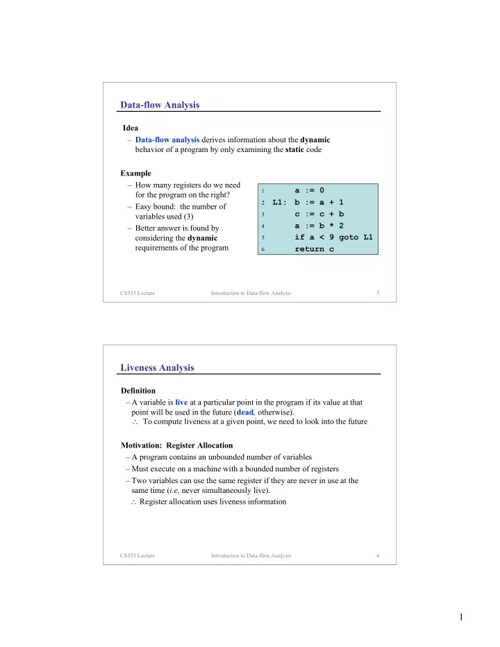
a := 0

2

L1: b := a + 1

3

c := c + b

4

a := b * 2

5

if a < 9 goto L1

6

return c Example – How many registers do we need for the program on the right? – Easy bound: the number of variables used (3) – Better answer is found by considering the dynamic requirements of the program

CS553 Lecture Introduction to Data-flow Analysis 4

Liveness Analysis

Definition

– A variable is live at a particular point in the program if its value at that point will be used in the future (dead, otherwise). ∴ To compute liveness at a given point, we need to look into the future

Motivation: Register Allocation

– A program contains an unbounded number of variables – Must execute on a machine with a bounded number of registers – Two variables can use the same register if they are never in use at the same time (i.e, never simultaneously live). ∴ Register allocation uses liveness information

2

CS553 Lecture Introduction to Data-flow Analysis 5

Liveness by Example

What is the live range of b?

– Variable b is read in statement 4, so b is live on the (3 → 4) edge – Since statement 3 does not assign into b, b is also live on the (2→3) edge – Statement 2 assigns b, so any value of b on the (1→2) and (5→ 2) edges are not needed, so b is dead along these edges

b’s live range is (2→3→4)

return c a = 0 b = a + 1 a<9

1 2 6 5 3 4 a = b * 2

c = c + b

Yes No CS553 Lecture Introduction to Data-flow Analysis 6

Liveness by Example (cont)

Live range of a

– a is live from (1→2) and again from (4→5→2) – a is dead from (2→3→4)

Live range of b

– b is live from (2→3→4)

Live range of c

– c is live from (entry→1→2→3→4→5→2, 5→6) return c a = 0 b = a + 1 a<9

1 2 6 5 3 4 a = b * 2

c = c + b

Yes No

Variables a and b are never simultaneously live, so they can share a register

3

CS553 Lecture Introduction to Data-flow Analysis 7

Control Flow Graphs (CFGs)

Definition

– A CFG is a graph whose nodes represent program statements and whose directed edges represent control flow

Example 1

a := 0

2

L1: b := a + 1

3

c := c + b

4

a := b * 2

5

if a < 9 goto L1

6

return c return c a = 0 b = a + 1 a<9

1 2 6 5 3 4 a = b * 2

c = c + b

Yes No CS553 Lecture Introduction to Data-flow Analysis 8

Terminology

Flow Graph Terms

– A CFG node has out-edges that lead to successor nodes and in-edges that come from predecessor nodes – pred[n] is the set of all predecessors of node n succ[n] is the set of all successors of node n

Examples

– Out-edges of node 5: – succ[5] = – pred[5] = – pred[2] = return c a = 0 b = a + 1 a<9

1 2 6 5 3 4 a = b * 2

c = c + b (5→6) and (5→2) {2,6} {1,5} {4}

Yes No

4

CS553 Lecture Introduction to Data-flow Analysis 9

Uses and Defs

Def (or definition)

– An assignment of a value to a variable – def[v] = set of CFG nodes that define variable v – def[n] = set of variables that are defined at node n

Use

– A read of a variable’s value – use[v] = set of CFG nodes that use variable v – use[n] = set of variables that are used at node n

More precise definition of liveness

– A variable v is live on a CFG edge if

a = 0 a < 9? ∉ def[v] ∈ use[v] v live

(1) ∃ a directed path from that edge to a use of v (node in use[v]), and

(2) that path does not go through any def of v (no nodes in def[v])

CS553 Lecture Introduction to Data-flow Analysis 10

a := b * 2

5

c := c + b

The Flow of Liveness

Data-flow

– Liveness of variables is a property that flows through the edges of the CFG

Direction of Flow

– Liveness flows backwards through the CFG, because the behavior at future nodes determines liveness at a given node – Consider a – Consider b – Later, we’ll see other properties that flow forward a < 9? b := a + 1

Yes No 3 1

a := 0

4 6

return c

2

5

CS553 Lecture Introduction to Data-flow Analysis 11

Liveness at Nodes

edges a = 0

Two More Definitions

– A variable is live-out at a node if it is live on any of that node’s out- edges – A variable is live-in at a node if it is live on any of that node’s in-edges

We have liveness on edges

– How do we talk about liveness at nodes? just after computation just before computation a := b * 2

5

c := c + b a < 9? b := a + 1

Yes No 3 1

a := 0

4 6

return c

2 n live-out

• ut-edges

n live-in in-edges

program points

CS553 Lecture Introduction to Data-flow Analysis 12

Data-flow equations in[n] = use[n] ∪ (out[n] – def[n])

• ut[n] = ∪ in[s]

s ∈ succ[n]

(1) (3) (2)

Rules for computing liveness (1) Generate liveness:

If a variable is in use[n], it is live-in at node n

n live-in use live-in n live-out

(3) Push liveness across nodes:

If a variable is live-out at node n and not in def[n] then the variable is also live-in at n

live-out n live-in pred[n] live-out live-out

(2) Push liveness across edges:

If a variable is live-in at a node n then it is live-out at all nodes in pred[n]

Computing Liveness

6

CS553 Lecture Introduction to Data-flow Analysis 13

Solving the Data-flow Equations

Algorithm This is iterative data-flow analysis (for liveness analysis)

for each node n in CFG in[n] = ∅; out[n] = ∅ repeat for each node n in CFG in’[n] = in[n]

• ut’[n] = out[n]

in[n] = use[n] ∪ (out[n] – def[n])

• ut[n] = ∪ in[s]

until in’[n]=in[n] and out’[n]=out[n] for all n

s ∈ succ[n]

initialize solutions solve data-flow equations test for convergence save current results

CS553 Lecture Introduction to Data-flow Analysis 14

3 bc c 5 a 2 a b 1 a node # use def in out in out in out in out in out in out in out 4 b a 6 c 1st 2nd 3rd 4th 5th 6th 7th c a b a a bc a c a bc bc b b a a ac a c ac bc bc b b a ac ac ac c ac bc bc b b ac ac ac c ac c ac bc bc b bc ac ac ac c ac c ac bc bc bc bc ac ac ac c ac c ac bc bc bc bc ac ac ac

Data-flow Equations for Liveness in[n] = use[n] ∪ (out[n] – def[n])

• ut[n] = ∪ in[s]

s ∈ succ[n] Yes No 2 b := a + 1 3 c := c + b 1

a := 0

4 a := b * 2 5

a < 9?

6

return c

Example

7

CS553 Lecture Introduction to Data-flow Analysis 15

Improving Performance Consider the (3→4) edge in the graph:

• ut[4] is used to compute in[4]

in[4] is used to compute out[3] . . . So we should compute the sets in the

• rder: out[4], in[4], out[3], in[3], . . .

Data-flow Equations for Liveness in[n] = use[n] ∪ (out[n] – def[n])

• ut[n] = ∪ in[s]

s ∈ succ[n]

The order of computation should follow the direction of flow

• ut[4]

in[4]

• ut[3]

Yes No 2 b := a + 1 3 c := c + b 1

a := 0

4 a := b * 2 5

a < 9?

6

return c

Example (cont)

CS553 Lecture Introduction to Data-flow Analysis 16

4 b a ac bc ac bc ac bc 2 a b bc ac bc ac bc ac 5 a c ac ac ac ac ac 1 a ac c ac c ac c 6 c c c c node # use def out in out in out in 3 bc c bc bc bc bc bc bc 1st 2nd 3rd

Converges much faster!

Yes No 2 b := a + 1 3 c := c + b 1

a := 0

4 a := b * 2 5

a < 9?

6

return c

Iterating Through the Flow Graph Backwards

8

CS553 Lecture Introduction to Data-flow Analysis 17

Solving the Data-flow Equations (reprise)

Algorithm

for each node n in CFG in[n] = ∅; out[n] = ∅ repeat for each node n in CFG in reverse topsort order in’[n] = in[n]

• ut’[n] = out[n]
• ut[n] = ∪ in[s]

in[n] = use[n] ∪ (out[n] – def[n]) until in’[n]=in[n] and out’[n]=out[n] for all n

s ∈ succ[n]

Initialize solutions Solve data-flow equations Test for convergence Save current results

CS553 Lecture Introduction to Data-flow Analysis 18

Time Complexity

Consider a program of size N

– Has N nodes in the flow graph and at most N variables – Each live-in or live-out set has at most N elements – Each set-union operation takes O(N) time – The for loop body – constant # of set operations per node – O(N) nodes ⇒ O(N2) time for the loop – Each iteration of the repeat loop can only make the set larger – Each set can contain at most N variables ⇒ 2N2 iterations

Worst case:

O(N4)

Typical case:

2 to 3 iterations with good ordering & sparse sets ⇒ O(N) to O(N2)

9

CS553 Lecture Introduction to Data-flow Analysis 19

More Performance Considerations

Basic blocks

– Decrease the size of the CFG by merging nodes that have a single predecessor and a single successor into basic blocks

One variable at a time

– Instead of computing data-flow information for all variables at once using sets, compute a (simplified) analysis for each variable separately

Representation of sets

– For dense sets, use a bit vector representation – For sparse sets, use a sorted list (e.g., linked list)

No 1

a := 0

3

return c

2 b := a + 1

c := c + 1 a := b * 2 a > 9?

Yes 2 3 Yes No

b := a + 1 c := c + b

4 a := b * 2 5

a < 9?

6

return c

1

a := 0

CS553 Lecture Introduction to Data-flow Analysis 20

3 bc c bc bc bcd bcd b b 5 a ac ac acd acd ac ac 2 a b ac bc acd bcd ac b 6 c c c c 1 a c ac cd acd c ac node # use def in out in out in out 4 b a bc ac bcd acd b ac X Y Z

Yes No 2 b := a + 1 3 c := c + b 1

a := 0

4 a := b * 2 5

a < 9?

6

return c

Conservative Approximation

Solution X

– Our solution as computed on previous slides

10

CS553 Lecture Introduction to Data-flow Analysis 21

3 bc c bc bc bcd bcd b b 5 a ac ac acd acd ac ac 2 a b ac bc acd bcd ac b 6 c c c c 1 a c ac cd acd c ac node # use def in out in out in out 4 b a bc ac bcd acd b ac X Y Z

Imprecise conservative solutions ⇒ sub-optimal but correct programs

Yes No 2 b := a + 1 3 1

a := 0

4 a := b * 2 5

a < 9?

6

return c

Conservative Approximation (cont)

Solution Y

– Carries variable d uselessly around the loop – Does Y solve the equations? – Is d live? – Does Y lead to a correct program? c := c + b

CS553 Lecture Introduction to Data-flow Analysis 22

3 bc c bc bc bcd bcd b b 5 a ac ac acd acd ac ac 2 a b ac bc acd bcd ac b 6 c c c c 1 a c ac cd acd c ac node # use def in out in out in out 4 b a bc ac bcd acd b ac X Y Z

Non-conservative solutions ⇒ incorrect programs

Yes No 1

a := 0

4 a := b * 2 5

a < 9?

6

return c

Conservative Approximation (cont)

Solution Z

– Does not identify c as live in all cases – Does Z solve the equations? – Does Z lead to a correct program? c := c + b b := a + 1

2 3

11

CS553 Lecture Introduction to Data-flow Analysis 23

No compiler can statically know all a program’s dynamic properties!

The Need for Approximations

Static vs. Dynamic Liveness

– In the following graph, b*b is always non-negative, so c >= b is always true and a’s value will never be used after node 2

Yes No 2 c := a + b 3

c >= b?

1 a := b * b 4

return a

5

return c Rule (2) for computing liveness – Since a is live-in at node 4, it is live-

• ut at nodes 3 and 2

– This rule ignores actual control flow

CS553 Lecture Introduction to Data-flow Analysis 24

Concepts

Liveness

– Use in register allocation – Generating liveness – Flow and direction – Data-flow equations and analysis – Complexity – Improving performance (basic blocks, single variable, bit sets)

Control flow graphs

– Predecessors and successors

Defs and uses Conservative approximation

– Static versus dynamic liveness

12

CS553 Lecture Introduction to Data-flow Analysis 25

Next Time

Reading

– Muchnick Ch. 7-7.5

Think about. . .

– Other data-flow analyses

Lecture

– Control-flow analysis – Basic blocks and control-flow graphs