1 Ways to improve data-flow analysis efficiency Example (liveness) - - PowerPoint PPT Presentation

1

CS553 Lecture Data-Flow Analysis Efficiency 1

Speeding Up Data-Flow Analysis

– Various optimizations that use data-flow analysis

– Speeding up data-flow analysis

CS553 Lecture Data-Flow Analysis Efficiency 2

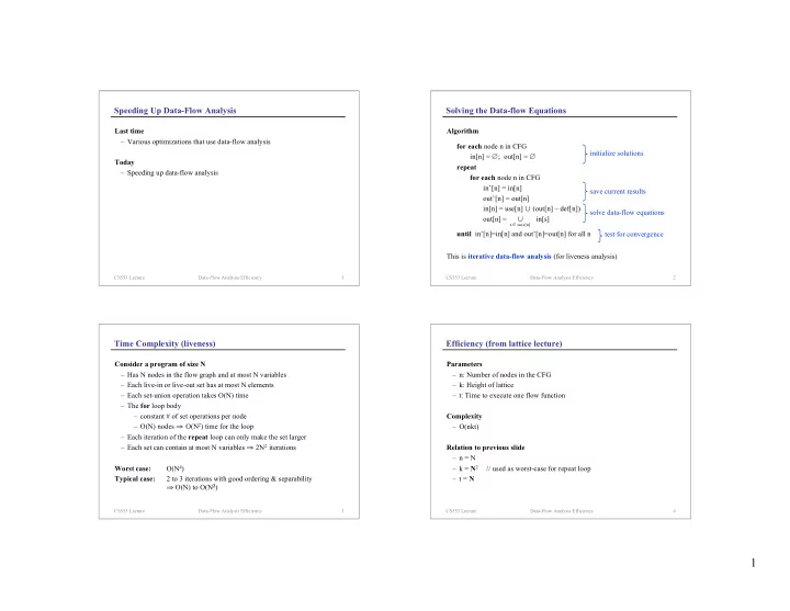
Solving the Data-flow Equations

for each node n in CFG in[n] = ∅; out[n] = ∅ repeat for each node n in CFG in’[n] = in[n]

• ut’[n] = out[n]

in[n] = use[n] ∪ (out[n] – def[n])

• ut[n] = ∪ in[s]

until in’[n]=in[n] and out’[n]=out[n] for all n

s ∈ succ[n]

initialize solutions solve data-flow equations test for convergence save current results

CS553 Lecture Data-Flow Analysis Efficiency 3

Time Complexity (liveness)

– Has N nodes in the flow graph and at most N variables – Each live-in or live-out set has at most N elements – Each set-union operation takes O(N) time – The for loop body – constant # of set operations per node – O(N) nodes ⇒ O(N2) time for the loop – Each iteration of the repeat loop can only make the set larger – Each set can contain at most N variables ⇒ 2N2 iterations

O(N4)

2 to 3 iterations with good ordering & separability ⇒ O(N) to O(N2)

CS553 Lecture Data-Flow Analysis Efficiency 4

Efficiency (from lattice lecture)

– n: Number of nodes in the CFG – k: Height of lattice – t: Time to execute one flow function

– O(nkt)

– n = N – k = N2 // used as worst-case for repeat loop – t = N

2

CS553 Lecture Data-Flow Analysis Efficiency 5

Ways to improve data-flow analysis efficiency

– Visit nodes in an ordering that most efficiently propagates change

– Use the tuple of lattices concept to implement the data-flow sets as bit-vectors

– Only visit nodes where the input data-flow sets have changed

– Group statements with straight-forward control-flow

– Structural or interval analysis – Slotwise analysis – SSA

CS553 Lecture Data-Flow Analysis Efficiency 6

3 bc c 5 a 2 a b 1 a node # use def in out in out in out in out in out in out in out 4 b a 6 c 1st 2nd 3rd 4th 5th 6th 7th c a b a a bc a c a bc bc b b a a ac a c ac bc bc b b a ac ac ac c ac bc bc b b ac ac ac c ac c ac bc bc b bc ac ac ac c ac c ac bc bc bc bc ac ac ac c ac c ac bc bc bc bc ac ac ac

Data-flow Equations for Liveness in[n] = use[n] ∪ (out[n] – def[n])

• ut[n] = ∪ in[s]

s ∈ succ[n] Yes No 2 b := a + 1 3 c := c + b 1

a := 0

4 a := b * 2 5

a < 9?

6

return c

Example (liveness)

CS553 Lecture Data-Flow Analysis Efficiency 7

Improving Performance Consider the (3→4) edge in the graph:

• ut[4] is used to compute in[4]

in[4] is used to compute out[3] . . . So we should compute the sets in the

• rder: out[4], in[4], out[3], in[3], . . .

Data-flow Equations for Liveness in[n] = use[n] ∪ (out[n] – def[n])

• ut[n] = ∪ in[s]

s ∈ succ[n]

The order of computation should follow the direction of flow

• ut[4]

in[4]

• ut[3]

Yes No 2 b := a + 1 3 c := c + b 1

a := 0

4 a := b * 2 5

a < 9?

6

return c

Example (cont)

CS553 Lecture Data-Flow Analysis Efficiency 8

4 b a ac bc ac bc ac bc 2 a b bc ac bc ac bc ac 5 a c ac ac ac ac ac 1 a ac c ac c ac c 6 c c c c node # use def out in out in out in 3 bc c bc bc bc bc bc bc 1st 2nd 3rd

Converges much faster!

Yes No 2 b := a + 1 3 c := c + b 1

a := 0

4 a := b * 2 5

a < 9?

6

return c

Iterating Through the Flow Graph Backwards

3

CS553 Lecture Data-Flow Analysis Efficiency 9

Solving the Data-flow Equations (reprise)

for each node n in CFG in[n] = ∅; out[n] = ∅ repeat for each node n in CFG in reverse post dfs order in’[n] = in[n]

• ut’[n] = out[n]
• ut[n] = ∪ in[s]

in[n] = use[n] ∪ (out[n] – def[n]) until in’[n]=in[n] and out’[n]=out[n] for all n

s ∈ succ[n]

Initialize solutions Solve data-flow equations Test for convergence Save current results

CS553 Lecture Data-Flow Analysis Efficiency 10

Effects on complexity

– Conservative upper bound is that each iteration will only make one set larger by one element. – A better approximation for separable analyses is height of the lattice (k) times the depth of the graph (Knuth 1971, depth is 2.75 on average). – Now repeat loop complexity is k instead of N2.

– For dense sets, use a bit vector representation

– Use the tuple of lattices concept to implement the data-flow sets as bit-vectors. – Now time to execute one flow function (t) is N/(wordsize).

– For sparse sets, use a sorted list (e.g., linked list)

– Only visit nodes where the input data-flow sets have changed. – Does not change complexity, but makes it unnecessary for convergence check iteration in IDFA.

CS553 Lecture Data-Flow Analysis Efficiency 11

Basic Blocks

– Decrease the size of the CFG by merging nodes that have a single predecessor and a single successor into basic blocks

No 1

a := 0

3

return c

2 b := a + 1

c := c + 1 a := b * 2 a > 9?

Yes 2 3 Yes No

b := a + 1 c := c + b

4 a := b * 2 5

a < 9?

6

return c

1

a := 0

CS553 Lecture Data-Flow Analysis Efficiency 12

Concepts

– Complexity analysis – Node ordering – Bit vector implementation – Basic blocks

4

CS553 Lecture Data-Flow Analysis Efficiency 13

Next Time

– Ch 18.1, 19.5

– Control dependence – Loops – Dominators