Introduction to Data-flow analysis Last Time Implementing a Mark - PDF document

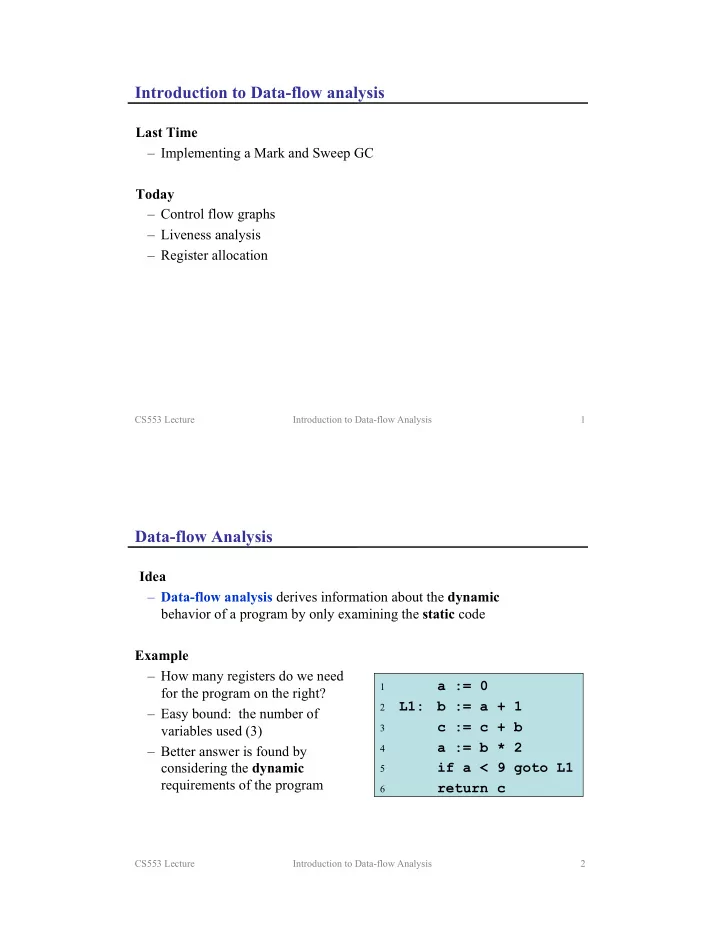
Introduction to Data-flow analysis � Last Time – � Implementing a Mark and Sweep GC � Today – � Control flow graphs – � Liveness analysis – � Register allocation CS553 Lecture Introduction to Data-flow Analysis 1 Data-flow Analysis � Idea – � Data-flow analysis derives information about the dynamic behavior of a program by only examining the static code Example – � How many registers do we need � 1 a := 0 for the program on the right? � 2 L1: b := a + 1 – � Easy bound: the number of � 3 c := c + b variables used (3) � 4 a := b * 2 – � Better answer is found by considering the dynamic � 5 if a < 9 goto L1 requirements of the program return c � 6 CS553 Lecture Introduction to Data-flow Analysis 2

Liveness Analysis � Definition – � A variable is live at a particular point in the program if its value at that point will be used in the future ( dead , otherwise). � To compute liveness at a given point, we need to look into the future � Motivation: Register Allocation – � A program contains an unbounded number of variables – � Must execute on a machine with a bounded number of registers – � Two variables can use the same register if they are never in use at the same time ( i.e, never simultaneously live). � Register allocation uses liveness information CS553 Lecture Introduction to Data-flow Analysis 3 Control Flow Graphs (CFGs) � Definition – � A CFG is a graph whose nodes represent program statements and whose directed edges represent control flow 1 a = 0 � Example � 1 a := 0 2 b = a + 1 � 2 L1: b := a + 1 � 3 c := c + b 3 c = c + b � 4 a := b * 2 4 a = b * 2 � 5 if a < 9 goto L1 � 6 return c 5 a<9 No Yes return c 6 CS553 Lecture Introduction to Data-flow Analysis 4

Terminology � Flow Graph Terms – � A CFG node has out-edges that lead to successor nodes and in-edges that come from predecessor nodes – � pred[n] is the set of all predecessors of node n 1 a = 0 succ[n] is the set of all successors of node n 2 b = a + 1 � Examples – � Out-edges of node 5: (5 � 6) and (5 � 2) 3 c = c + b {2,6} – � succ[5] = – � pred[5] = {4} 4 a = b * 2 {1,5} – � pred[2] = 5 a<9 No Yes return c 6 CS553 Lecture Introduction to Data-flow Analysis 5 Liveness by Example � What is the live range of b ? – � Variable b is read in statement 4, 1 a = 0 so b is live on the (3 � 4) edge – � Since statement 3 does not assign 2 b = a + 1 into b , b is also live on the (2 � 3) edge 3 c = c + b – � Statement 2 assigns b , so any value of b on the (1 � 2) and 4 a = b * 2 (5 � 2) edges are not needed, so b is dead along these edges 5 a<9 No Yes � b ’s live range is (2 � 3 � 4) return c 6 CS553 Lecture Introduction to Data-flow Analysis 6

Liveness by Example (cont) � Live range of a – � a is live from (1 � 2) and again from 1 a = 0 (4 � 5 � 2) – � a is dead from (2 � 3 � 4) 2 b = a + 1 � Live range of b 3 c = c + b – � b is live from (2 � 3 � 4) 4 a = b * 2 � Live range of c – � c is live from a<9 5 (entry � 1 � 2 � 3 � 4 � 5 � 2, 5 � 6) No Yes return c 6 Variables a and b are never simultaneously live, so they can share a register � CS553 Lecture Introduction to Data-flow Analysis 7 Uses and Defs � Def (or definition) a = 0 – � An assignment of a value to a variable – � def_node[v] = set of CFG nodes that define variable v – � def[n] = set of variables that are defined at node n a < 9? � Use – � A read of a variable’s value v live – � use_node[v] = set of CFG nodes that use variable v – � use[n] = set of variables that are used at node n � def_node[v] � More precise definition of liveness � use_node[v] – � A variable v is live on a CFG edge if � (1) � a directed path from that edge to a use of v (node in use_node[v]), and (2) that path does not go through any def of v (no nodes in def_node[v]) CS553 Lecture Introduction to Data-flow Analysis 8

The Flow of Liveness � Data-flow – � Liveness of variables is a property that flows through the edges of the CFG a := 0 1 � Direction of Flow 2 b := a + 1 – � Liveness flows backwards through the CFG, because the behavior at future nodes c := c + b 3 determines liveness at a given node a := b * 2 4 – � Consider a – � Consider b a < 9? 5 – � Later, we’ll see other properties No Yes that flow forward return c 6 CS553 Lecture Introduction to Data-flow Analysis 9 program points Liveness at Nodes edges � We have liveness on edges just before computation a = 0 – � How do we talk about just after computation liveness at nodes? � Two More Definitions – � A variable is live-out at a node if it is live on any of that node’s out-edges n live-out out-edges – � A variable is live-in at a node if it is live on any of that node’s in-edges in-edges n live-in CS553 Lecture Introduction to Data-flow Analysis 10

Computing Liveness � Rules for computing liveness � (1) Generate liveness: live-in n use If a variable is in use[n], it is live-in at node n � (2) Push liveness across edges: pred[n] live-out live-out live-out If a variable is live-in at a node n then it is live-out at all nodes in pred[n] n live-in � � (3) Push liveness across nodes: If a variable is live-out at node n and not in def[n] live-in n then the variable is also live-in at n � live-out � Data-flow equations (1) in[n] = use[n] � (out[n] – def[n]) � (3) out[n] = � in[s] � (2) s � succ[n] CS553 Lecture Introduction to Data-flow Analysis 11 Solving the Data-flow Equations � Algorithm for each node n in CFG initialize solutions in[n] = � ; out[n] = � repeat for each node n in CFG in’[n] = in[n] save current results out’[n] = out[n] in[n] = use[n] � (out[n] – def[n]) solve data-flow equations out[n] = � in[s] s � succ[n] test for convergence until in’[n]=in[n] and out’[n]=out[n] for all n � This is iterative data-flow analysis (for liveness analysis) CS553 Lecture Introduction to Data-flow Analysis 12

Example 1st 2nd 3rd 4th 5th 6th 7th node use def in out in out in out in out in out in out in out # a := 0 1 1 a a a ac c ac c ac c ac 2 a b a a bc ac bc ac bc ac bc ac bc ac bc 2 b := a + 1 bc 3 bc c bc b bc b bc b bc b bc bc bc bc 4 b a b b a b ac bc ac bc ac bc ac 3 c := c + b b a a ac ac ac 5 a a a ac ac ac ac ac ac ac ac 4 a := b * 2 6 c c c c c c c c a < 9? Data-flow Equations for Liveness 5 No Yes in[n] = use[n] � (out[n] – def[n]) return c 6 out[n] = � in[s] s � succ[n] CS553 Lecture Introduction to Data-flow Analysis 13 Liveness Analysis in the MiniJava compiler � Currently … – � Parse into AST – � Allocate space on stack for locals and parameters and space in heap for member variables – � Use stack for expression evaluation – � Generate MIPS code from AST � To perform data-flow analysis … – � Need intermediate representation like 3-address code – � Use temporaries for parameters, locals, and expression results – � Indicate uses and defs of temporaries in each 3-address code instruction – � Create a control-flow graph with each 3-address code instruction as a node CS553 Lecture Introduction to Data-flow Analysis 14

Register Allocation Problem � – � Assign an unbounded number of symbolic registers to a fixed number of architectural registers – � Simultaneously live data must be assigned to different architectural registers Goal � – � Minimize overhead of accessing data – � Memory operations (loads & stores) – � Register moves CS553 Lecture Register Allocation I 15 Scope of Register Allocation Expression � Local � Loop � Global � Interprocedural � CS553 Lecture Register Allocation I 16

Granularity of Allocation What is allocated to registers? � – � Variables – � Live ranges/Webs ( i.e., du-chains with common uses) – � Values ( i.e., definitions; same as variables with SSA) s 1 : x := 5 b 1 Variables: 2 ( x & y ) Live Ranges/Web: 3 (s 1 � s 2 ,s 4 ; s 2 : y := x s 4 : ... x ... s 2 � s 3 ; b 2 b 3 s 3 : x := y+1 s 5 : x := 3 s 3 ,s 5 � s 6 ) Values: 4 (s 1 , s 2 , s 3 , s 5 , � (s 3 ,s 5 )) s 6 : ... x ... b 4 What are the tradeoffs? Each allocation unit is given a symbolic register name (e.g., t1 , t2 , etc.) CS553 Lecture Register Allocation I 17 Global Register Allocation by Graph Coloring Idea [Cocke 71], First allocator [Chaitin 81] 1. � Construct interference graph G=(N,E) – � Represents notion of “simultaneously live” – � Nodes are units of allocation ( e.g., variables, live ranges, values) – � � edge (n 1 ,n 2 ) � E if n 1 and n 2 are simultaneously live – � Symmetric (not reflexive nor transitive) 2. � Find k -coloring of G (for k registers) – � Adjacent nodes can’t have same color 3. Allocate the same register to all allocation units of the same color – � Adjacent nodes must be allocated to distinct registers t2 t1 t3 CS553 Lecture Register Allocation I 18