1 Liveness by Example (cont) Control Flow Graphs (CFGs) Live range - - PowerPoint PPT Presentation

1

CS553 Lecture Introduction to Data-flow Analysis 2

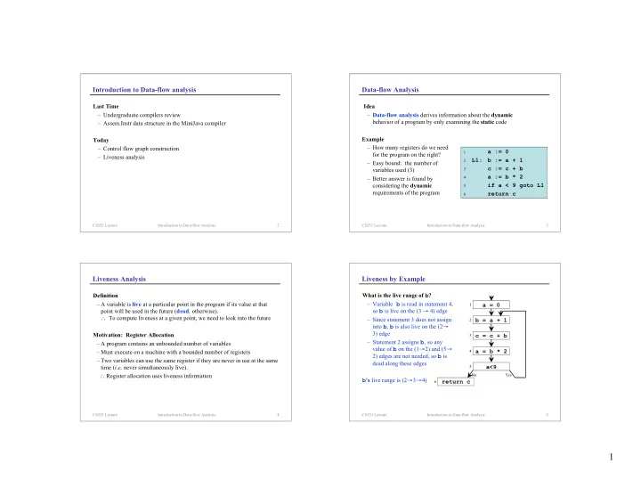
Introduction to Data-flow analysis

– Undergraduate compilers review – Assem.Instr data structure in the MiniJava compiler

– Control flow graph construction – Liveness analysis

CS553 Lecture Introduction to Data-flow Analysis 3

Data-flow Analysis

– Data-flow analysis derives information about the dynamic behavior of a program by only examining the static code

a := 0

L1: b := a + 1

c := c + b

a := b * 2

if a < 9 goto L1

return c Example – How many registers do we need for the program on the right? – Easy bound: the number of variables used (3) – Better answer is found by considering the dynamic requirements of the program

CS553 Lecture Introduction to Data-flow Analysis 4

Liveness Analysis

– A variable is live at a particular point in the program if its value at that point will be used in the future (dead, otherwise). ∴ To compute liveness at a given point, we need to look into the future

– A program contains an unbounded number of variables – Must execute on a machine with a bounded number of registers – Two variables can use the same register if they are never in use at the same time (i.e, never simultaneously live). ∴ Register allocation uses liveness information

CS553 Lecture Introduction to Data-flow Analysis 5

Liveness by Example

– Variable b is read in statement 4, so b is live on the (3 → 4) edge – Since statement 3 does not assign into b, b is also live on the (2→ 3) edge – Statement 2 assigns b, so any value of b on the (1→2) and (5→ 2) edges are not needed, so b is dead along these edges

return c a = 0 b = a + 1 a<9

1 2 6 5 3 4 a = b * 2

c = c + b

Yes No

2

CS553 Lecture Introduction to Data-flow Analysis 6

Liveness by Example (cont)

– a is live from (1→2) and again from (4→5→2) – a is dead from (2→3→4)

– b is live from (2→3→4)

– c is live from (entry→1→2→3→4→5→2, 5→6) return c a = 0 b = a + 1 a<9

1 2 6 5 3 4 a = b * 2

c = c + b

Yes No

Variables a and b are never simultaneously live, so they can share a register

CS553 Lecture Introduction to Data-flow Analysis 7

Control Flow Graphs (CFGs)

– A CFG is a graph whose nodes represent program statements and whose directed edges represent control flow

a := 0

L1: b := a + 1

c := c + b

a := b * 2

if a < 9 goto L1

return c return c a = 0 b = a + 1 a<9

1 2 6 5 3 4 a = b * 2

c = c + b

Yes No CS553 Lecture Introduction to Data-flow Analysis 8

Terminology

– A CFG node has out-edges that lead to successor nodes and in-edges that come from predecessor nodes – pred[n] is the set of all predecessors of node n succ[n] is the set of all successors of node n

– Out-edges of node 5: – succ[5] = – pred[5] = – pred[2] = return c a = 0 b = a + 1 a<9

1 2 6 5 3 4 a = b * 2

c = c + b (5→6) and (5→2) {2,6} {1,5} {4}

Yes No CS553 Lecture Introduction to Data-flow Analysis 9

Uses and Defs

– An assignment of a value to a variable – def[v] = set of CFG nodes that define variable v – def[n] = set of variables that are defined at node n

– A read of a variable’s value – use[v] = set of CFG nodes that use variable v – use[n] = set of variables that are used at node n

– A variable v is live on a CFG edge if

a = 0 a < 9? ∉ def[v] ∈ use[v] v live

(2) that path does not go through any def of v (no nodes in def[v])

3

CS553 Lecture Introduction to Data-flow Analysis 10

a := b * 2

5

c := c + b

The Flow of Liveness

– Liveness of variables is a property that flows through the edges of the CFG

– Liveness flows backwards through the CFG, because the behavior at future nodes determines liveness at a given node – Consider a – Consider b – Later, we’ll see other properties that flow forward a < 9? b := a + 1

Yes No 3 1

a := 0

4 6

return c

2 CS553 Lecture Introduction to Data-flow Analysis 11

Liveness at Nodes

edges a = 0

– A variable is live-out at a node if it is live on any of that node’s out- edges – A variable is live-in at a node if it is live on any of that node’s in-edges

– How do we talk about liveness at nodes? just after computation just before computation

n live-out

• ut-edges

n live-in in-edges

program points

CS553 Lecture Introduction to Data-flow Analysis 12

Data-flow equations in[n] = use[n] ∪ (out[n] – def[n])

• ut[n] = ∪ in[s]

s ∈ succ[n]

(1) (3) (2)

If a variable is in use[n], it is live-in at node n

n live-in use live-in n live-out

If a variable is live-out at node n and not in def[n] then the variable is also live-in at n

live-out n live-in pred[n] live-out live-out

If a variable is live-in at a node n then it is live-out at all nodes in pred[n]

Computing Liveness

CS553 Lecture Introduction to Data-flow Analysis 13

Solving the Data-flow Equations

for each node n in CFG in[n] = ∅; out[n] = ∅ repeat for each node n in CFG in’[n] = in[n]

• ut’[n] = out[n]

in[n] = use[n] ∪ (out[n] – def[n])

• ut[n] = ∪ in[s]

until in’[n]=in[n] and out’[n]=out[n] for all n

s ∈ succ[n]

initialize solutions solve data-flow equations test for convergence save current results

4

CS553 Lecture Introduction to Data-flow Analysis 14

3 bc c 5 a 2 a b 1 a node # use def in out in out in out in out in out in out in out 4 b a 6 c 1st 2nd 3rd 4th 5th 6th 7th c a b a a bc a c a bc bc b b a a ac a c ac bc bc b b a ac ac ac c ac bc bc b b ac ac ac c ac c ac bc bc b bc ac ac ac c ac c ac bc bc bc bc ac ac ac c ac c ac bc bc bc bc ac ac ac

Data-flow Equations for Liveness in[n] = use[n] ∪ (out[n] – def[n])

• ut[n] = ∪ in[s]

s ∈ succ[n] Yes No 2 b := a + 1 3 c := c + b 1

a := 0

4 a := b * 2 5

a < 9?

6

return c

Example

CS553 Lecture Introduction to Data-flow Analysis 15

Liveness in the MiniJava compiler

CS553 Lecture Introduction to Data-flow Analysis 16

Concepts

– Used in register allocation – Generating liveness – Flow and direction – Data-flow equations and analysis

– Predecessors and successors

CS553 Lecture Introduction to Data-flow Analysis 17

Next Time

– Ch 11, register allocation

– Register allocation