D ilute Solution C hain D ynam ics of the chain T he exponential - - PowerPoint PPT Presentation

d ilute solution c hain d ynam ics of the chain
SMART_READER_LITE
LIVE PREVIEW

D ilute Solution C hain D ynam ics of the chain T he exponential - - PowerPoint PPT Presentation

D ilute Solution C hain D ynam ics of the chain T he exponential term is the response function response to a pulse perturbation 1 D ilute Solution C hain D ynam ics of the chain D am ped H arm onic O scillator For Brow nian m otion


slide-1
SLIDE 1

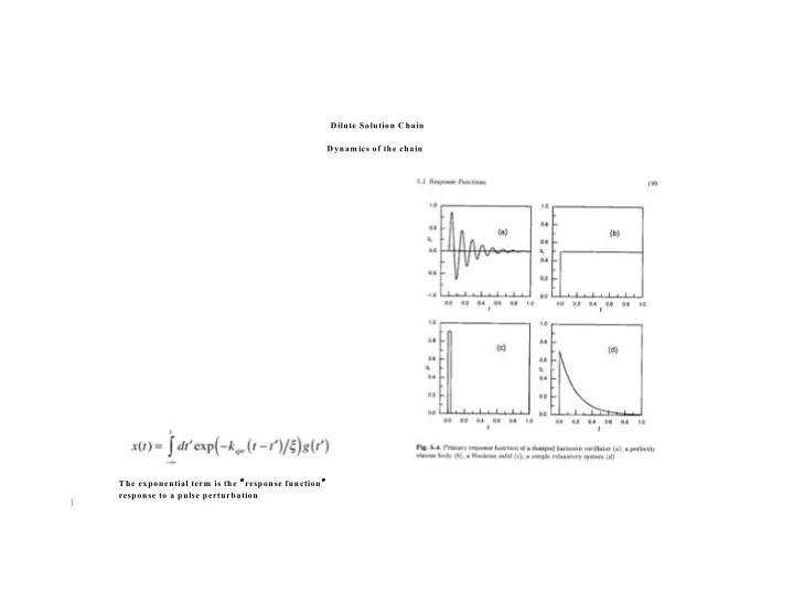
1 D ilute Solution C hain D ynam ics of the chain T he exponential term is the response function response to a pulse perturbation

slide-2
SLIDE 2

2 D ilute Solution C hain D ynam ics of the chain D am ped H arm onic O scillator For Brow nian m otion

  • f a harm onic bead in a solvent

this response function can be used to calculate the tim e correlation function <x(t)x(0)> for DLS for instance τ is a relaxation tim e.

slide-3
SLIDE 3

Draining vs Non Draining Rouse vs Zimm Consider Diffusion of a Chain D = kT/z For Non Draining

slide-4
SLIDE 4
slide-5
SLIDE 5

5

Dilute Solution Chain Dynamics of the chain Rouse Motion Beads 0 and N are special For Beads 1 to N-1 For Bead 0 use R-1 = R0 and for bead N RN+1 = RN This is called a closure relationship

slide-6
SLIDE 6

6

Dilute Solution Chain Dynamics of the chain Rouse Motion The Rouse unit size is arbitrary so we can make it very small and: With dR/dt = 0 at i = 0 and N Reflects the curvature of R in i, it describes modes of vibration like on a guitar string

slide-7
SLIDE 7

7

Dilute Solution Chain Dynamics of the chain Rouse Motion Describes modes of vibration like on a guitar string For the pth mode (0th mode is the whole chain (string))

slide-8
SLIDE 8

8

x, y, z decouple (are equivalent) so you can just deal with z For a chain of infinite molecular weight there are wave solutions to this series of differential equations

ς R dzl dt = bR(zl+1 − zl)+ bR(zl

−1 − zl)

zl ~ exp − t τ ⎛ ⎝ ⎜ ⎞ ⎠ ⎟ exp ilδ

( )

τ −1 = bR ζ R 2 − 2cosδ

( ) = 4bR

ζ R sin2 δ 2

slide-9
SLIDE 9

9

τ −1 = bR ζ R 2 − 2cosδ

( ) = 4bR

ζ R sin2 δ 2

Cyclic Boundary Conditions:

zl = zl+NR NRδ = m2π

NR values of phase shift

δm = 2π NR m; m = − NR 2 −1 ⎛ ⎝ ⎜ ⎞ ⎠ ⎟,..., NR 2

For NR = 10

slide-10
SLIDE 10

1 0

τ −1 = bR ζ R 2 − 2cosδ

( ) = 4bR

ζ R sin2 δ 2

Free End Boundary Conditions:

zl − z0 = zNR−1 − zNR−2 = 0 NR −1

( )δ = mπ

NR values of phase shift

δm = π NR −1

( )

m; m = 0,1,2,..., NR −1

( )

For NR = 10

dz dl l = 0

( ) = dz

dl l = NR −1

( ) = 0

NR Rouse Modes of order “m”

slide-11
SLIDE 11

1 1

τ R = 1 3π 2 ζ R aR

2

⎛ ⎝ ⎜ ⎞ ⎠ ⎟ kT R0

4

Lowest order relaxation time dominates the response This assumes that ζ R aR

2

⎛ ⎝ ⎜ ⎞ ⎠ ⎟ is constant, friction coefficient is proportional to number of monomer units in a Rouse segment This is the basic assumption of the Rouse model, ζ R ~ aR

2 ~ N

NR = nR

slide-12
SLIDE 12

1 2

τ R = 1 3π 2 ζ R aR

2

⎛ ⎝ ⎜ ⎞ ⎠ ⎟ kT R0

4

Lowest order relaxation time dominates the response Since

R0

2 = a0 2N

τ R ~ N 2 kT

slide-13
SLIDE 13

1 3

The amplitude of the Rouse modes is given by:

Zm

2 =

2 3π 2 R0

2

m2

The amplitude is independent of temperature because the free energy of a mode is proportional to kT and the modes are distributed by Boltzmann statistics

p Zm

( ) = exp − F

kT ⎛ ⎝ ⎜ ⎞ ⎠ ⎟

90% of the total mean-square end to end distance of the chain originates from the lowest order Rouse-modes so the chain can be often represented as an elastic dumbbell

slide-14
SLIDE 14

1 4

Rouse dynamics (like a dumbell response)

dx dt = − dU dx ⎛ ⎝ ⎜ ⎞ ⎠ ⎟ ζ + g(t) = − ksprx ζ + g(t) x t

( ) =

dt'exp − t − t' τ ⎛ ⎝ ⎜ ⎞ ⎠ ⎟

−∞ t

g t

( )

τ = ζ kspr

Dumbbell Rouse

τ R = ζ R 4bR sin2 δ 2 δ = π NR −1m , m=0,1,2,...,NR-1

slide-15
SLIDE 15

1 5

Rouse dynamics (like a dumbell response)

g t1

( )g t2 ( ) = 2Dδ t ( ) where t = t1 − t2 and δ ( ) is the delta function whose integral is 1

Also,

D = kT ζ x t

( )x 0 ( ) =

kT exp − t τ ⎛ ⎝ ⎜ ⎞ ⎠ ⎟ kspr τ = ζ kspr

For t => 0,

x2 = kT kspr

slide-16
SLIDE 16

1 6

Predictions of Rouse Model

G t

( ) ~ t

−1 2

G' ω

( ) ~ ωη0 ( )

1 2

η0 = kTρpτ R π 2 12 ~ N

slide-17
SLIDE 17

1 7

Dilute Solution Chain Dynamics of the chain Rouse Motion Rouse model predicts Relaxation time follows N2 (actually follows N3/df) Diffusion constant follows 1/N (zeroth order mode is translation of the molecule) (actually follows N-1/df) Both failings are due to hydrodynamic interactions (incomplete draining of coil) Predicts that the viscosity will follow N which is true for low molecular weights in the melt and for fully draining polymers in solution

slide-18
SLIDE 18

1 8

Dilute Solution Chain Dynamics of the chain Rouse Motion Rouse model predicts Relaxation time follows N2 (actually follows N3/df) Predicts that the viscosity will follow N which is true for low molecular weights in the melt and for fully draining polymers in solution