[PPT] - CSE 421: Algorithms and Computational Complexity Outline: General PowerPoint Presentation

SLIDE 1

1

CSE 421: Algorithms and Computational Complexity

Summer 2007 Larry Ruzzo

Divide and Conquer Algorithms

2

The Divide and Conquer Paradigm

Outline:

General Idea Review of Merge Sort Why does it work?

Importance of balance Importance of super-linear growth

Two interesting applications

Polynomial Multiplication Matrix Multiplication

Finding & Solving Recurrences

3

Algorithm Design Techniques

Divide & Conquer

Reduce problem to one or more sub-problems of the same type Typically, each sub-problem is at most a constant fraction of the size of the original problem

e.g. Mergesort, Binary Search, Strassen’s Algorithm, Quicksort (kind of)

4

Mergesort (review)

Mergesort: (recursively) sort 2 half-lists, then merge results. T(n)=2T(n/2)+cn, n≥2 T(1)=0 Solution: O(n log n) (details later)

Log n levels O(n) work per level

SLIDE 2

2

9

Why Balanced Subdivision?

Alternative "divide & conquer" algorithm: Sort n-1 Sort last 1 Merge them T(n)=T(n-1)+T(1)+3n for n ≥ 2 T(1)=0 Solution: 3n + 3(n-1) + 3(n-2) … = Θ(n2)

10

Suppose we've already invented DumbSort, taking time n2 Try Just One Level of divide & conquer:

DumbSort(first n/2 elements) DumbSort(last n/2 elements) Merge results

Time: 2 (n/2)2 + n = n2/2 + n << n2

Almost twice as fast!

Another D&C Approach

D&C in a nutshell

11

Another D&C Approach, cont.

Moral 1: “two halves are better than a whole”

Two problems of half size are better than one full-size problem, even given the O(n) overhead of recombining, since the base algorithm has super-linear complexity.

Moral 2: “If a little's good, then more's better”

two levels of D&C would be almost 4 times faster, 3 levels almost 8, etc., even though overhead is growing. Best is usually full recursion down to some small constant size (balancing "work" vs "overhead").

12

Another D&C Approach, cont.

Moral 3: unbalanced division less good:

(.1n)2 + (.9n)2 + n = .82n2 + n

The 18% savings compounds significantly if you carry recursion to more levels, actually giving O(nlogn), but with a bigger constant. So worth doing if you can’t get 50-50 split, but balanced is better if you can. This is intuitively why Quicksort with random splitter is good – badly unbalanced splits are rare, and not instantly fatal.

(1)2 + (n-1)2 + n = n2 - 2n + 2 + n

Little improvement here.

SLIDE 3

3 5.4 Closest Pair of Points

14

Closest Pair of Points

Closest pair. Given n points in the plane, find a pair with smallest Euclidean distance between them. Fundamental geometric primitive.

 Graphics, computer vision, geographic information systems,

molecular modeling, air traffic control.

 Special case of nearest neighbor, Euclidean MST, Voronoi.

Brute force. Check all pairs of points p and q with Θ(n2) comparisons. 1-D version. O(n log n) easy if points are on a line.

Assumption. No two points have same x coordinate.

to make presentation cleaner fast closest pair inspired fast algorithms for these problems

15

Closest Pair of Points: First Attempt

Divide. Sub-divide region into 4 quadrants.

L

16

Closest Pair of Points: First Attempt

Divide. Sub-divide region into 4 quadrants.
Obstacle. Impossible to ensure n/4 points in each piece.

L

SLIDE 4

4

17

Closest Pair of Points

Algorithm.

 Divide: draw vertical line L so that roughly ½n points on each side.

L

18

Closest Pair of Points

Algorithm.

 Divide: draw vertical line L so that roughly ½n points on each side.  Conquer: find closest pair in each side recursively.

12 21 L

19

Closest Pair of Points

Algorithm.

 Divide: draw vertical line L so that roughly ½n points on each side.  Conquer: find closest pair in each side recursively.  Combine: find closest pair with one point in each side.  Return best of 3 solutions.

12 21 8 L

seems like Θ(n2)

20

Closest Pair of Points

Find closest pair with one point in each side, assuming that distance < δ. 12 21 δ = min(12, 21) L

SLIDE 5

5

21

Closest Pair of Points

Find closest pair with one point in each side, assuming that distance < δ.

 Observation: only need to consider points within δ of line L.

12 21 δ L δ = min(12, 21)

22

12 21

1 2 3 4 5 6 7

δ

Closest Pair of Points

Find closest pair with one point in each side, assuming that distance < δ.

 Observation: only need to consider points within δ of line L.  Sort points in 2δ-strip by their y coordinate.

L δ = min(12, 21)

23

12 21

1 2 3 4 5 6 7

δ

Closest Pair of Points

Find closest pair with one point in each side, assuming that distance < δ.

 Observation: only need to consider points within δ of line L.  Sort points in 2δ-strip by their y coordinate.  Only check distances of those within 8 positions in sorted list!

L δ = min(12, 21)

24

Closest Pair of Points

Def. Let si be the point in the 2δ-strip, with

the ith smallest y-coordinate.

Claim. If |i – j| ≥ 8, then the distance between

si and sj is at least δ. Pf.

 No two points lie in same ½δ-by-½δ box.  only 8 boxes

δ

29 30 31 28 26 25

δ

½δ ½δ

39

i j

27

SLIDE 6

6

25

Closest Pair Algorithm

Closest-Pair(p1, …, pn) { if(n <= ??) return ?? Compute separation line L such that half the points are on one side and half on the other side. δ1 = Closest-Pair(left half) δ2 = Closest-Pair(right half) δ = min(δ1, δ2) Delete all points further than δ from separation line L Sort remaining points p[1]…p[m] by y-coordinate. for i = 1..m k = 1 while i+k <= m && p[i+k].y < p[i].y + δ δ = min(δ, distance between p[i] and p[i+k]); k++; return δ. }

26

Going From Code to Recurrence

Carefully define what you’re counting, and write it down!

“Let C(n) be the number of comparisons between sort keys used by MergeSort when sorting a list of length n ≥ 1”

In code, clearly separate base case from recursive case, highlight recursive calls, and operations being counted. Write Recurrence(s)

27

Closest Pair Algorithm

Closest-Pair(p1, …, pn) { if(n <= 1) return ∞ Compute separation line L such that half the points are on one side and half on the other side. δ1 = Closest-Pair(left half) δ2 = Closest-Pair(right half) δ = min(δ1, δ2) Delete all points further than δ from separation line L Sort remaining points p[1]…p[m] by y-coordinate. for i = 1..m k = 1 while i+k <= m && p[i+k].y < p[i].y + δ δ = min(δ, distance between p[i] and p[i+k]); k++; return δ. }

2T(n / 2) O(n)

Base Case Recursive calls (2) Basic operations at this recursive level Basic operations: distance calcs

28

Closest Pair of Points: Analysis

Running time. BUT - that’s only the number of distance calculations

T(n) n =1 2T n /2

( ) + 7n

n >1

T(n) = O(n logn)

SLIDE 7

7

29

Closest Pair Algorithm

Closest-Pair(p1, …, pn) { if(n <= 1) return ∞ Compute separation line L such that half the points are on one side and half on the other side. δ1 = Closest-Pair(left half) δ2 = Closest-Pair(right half) δ = min(δ1, δ2) Delete all points further than δ from separation line L Sort remaining points p[1]…p[m] by y-coordinate. for i = 1..m k = 1 while i+k <= m && p[i+k].y < p[i].y + δ δ = min(δ, distance between p[i] and p[i+k]); k++; return δ. }

O(n log n) 2T(n / 2) O(n) O(n log n) O(n)

Base Case Recursive calls (2) Basic operations at this recursive level Basic operations: comparisons 1

30

Closest Pair of Points: Analysis

Running time.

Q. Can we achieve O(n log n)?
A. Yes. Don't sort points from scratch each time.

 Sort by x at top level only.  Each recursive call returns δ and list of all points sorted by y  Sort by merging two pre-sorted lists.

T(n) 2T n/2

( ) + O(n)

T(n) = O(n logn)

T(n) n =1 2T n /2

( ) + O(n logn)

n >1

T(n) = O(n log2 n)

5.5 Integer Multiplication

32

Integer Arithmetic

Add. Given two n-digit integers a and b, compute a + b.

 O(n) bit operations.

Multiply. Given two n-digit integers a and b, compute a × b.

 Brute force solution: Θ(n2) bit operations.

1 1 1 1 1 1 1 1 1 1 1 1 1 1 1 1 1 1 1 1 1 1 1 1 1 1 1 1 1 1 1 1 1 1 1 1 1 1 1 1 1 1 1 1 1 * 1 1 1 1 1 1 1 + 1 1 1 1 1 1 1 1 1 1 1 1 1 1 1

Add Multiply

SLIDE 8

8

33

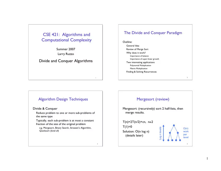
To multiply two n-digit integers:

 Multiply four ½n-digit integers.  Add two ½n-digit integers, and shift to obtain result.

Divide-and-Conquer Multiplication: Warmup

T(n) = 4T n/2

( )

recursive calls

1 2 4 3 4 + (n)

add, shift

1 2 3 T(n) = (n2)

x = 2n / 2 x1 + x0 y = 2n / 2 y1 + y0 xy = 2n / 2 x1 + x0

( ) 2n / 2 y1 + y0 ( )

= 2n x1y1 + 2n / 2 x1y0 + x0y1

( ) + x0y0

assumes n is a power of 2

1 1 1 1 1 1 1 1 1 1 1 1 1 1 1 * 1 1 1 1 1 1 1 1 1 1 1 1 1 1 x0⋅y0 x0⋅y1 x1⋅y0 x1⋅y1 x1 x0 y1 y0

34

Key trick: 2 multiplies for the price of 1:

x = 2n / 2 x1 + x0 y = 2n / 2 y1 + y0 xy = 2n / 2 x1 + x0

( ) 2n / 2 y1 + y0 ( )

= 2n x1y1 + 2n / 2 x1y0 + x0y1

( ) + x0y0

=

x1 + x0

=

y1 + y0

=

x1 + x0

( ) y1 + y0 ( )

= x1y1 + x1y0 + x0y1

( ) + x0y0

x1y0 + x0y1

( )

= x1y1 x0y0

Well, ok, 4 for 3 is more accurate…

35

To multiply two n-digit integers:

 Add two ½n digit integers.  Multiply three ½n-digit integers.  Add, subtract, and shift ½n-digit integers to obtain result.

Theorem. [Karatsuba-Ofman, 1962] Can multiply two n-digit integers

in O(n1.585) bit operations.

Karatsuba Multiplication

x = 2n /2 x1 + x0 y = 2n /2 y1 + y0 xy = 2n x1y1 + 2n /2 x1y0 + x0y1

( ) + x0y0

= 2n x1y1 + 2n /2 (x1 + x0)(y1 + y0) x1y1 x0y0

( ) + x0y0

T(n) T n /2

(

) + T

n /2

(

) + T 1+ n /2

(

)

recursive calls

1 2 4 4 4 4 4 4 4 3 4 4 4 4 4 4 4 + (n)

add, subtract, shift

1 2 4 3 4 Sloppy version : T(n) 3T(n /2) + O(n) T(n) = O(n

log 2 3 ) = O(n1.585 )

A B C A C

36

Multiplication – The Bottom Line

Naïve: Θ(n2) Karatsuba: Θ(n1.59…) Amusing exercise: generalize Karatsuba to do 5 size n/3 subproblems => Θ(n1.46…) Best known: Θ(n log n loglog n)

"Fast Fourier Transform" but mostly unused in practice (unless you need really big numbers - a billion digits of π, say)

High precision arithmetic IS important for crypto

SLIDE 9

9

37

Recurrences

Where they come from, how to find them (above) Next: how to solve them

38

Mergesort (review)

Mergesort: (recursively) sort 2 half-lists, then merge results. T(n)=2T(n/2)+cn, n≥2 T(1)=0 Solution: Θ(n log n)

(details later) Log n levels O(n) work per level

now

39

Merge Sort

MS(A: array[1..n]) returns array[1..n] {

If(n=1) return A[1]; New U:array[1:n/2] = MS(A[1..n/2]); New L:array[1:n/2] = MS(A[n/2+1..n]); Return(Merge(U,L)); }

Merge(U,L: array[1..n]) {

New C: array[1..2n]; a=1; b=1; For i = 1 to 2n C[i] = “smaller of U[a], L[b] and correspondingly a++ or b++”; Return C; }

A U C L split sort merge

40

Going From Code to Recurrence

Carefully define what you’re counting, and write it down!

“Let C(n) be the number of comparisons between sort keys used by MergeSort when sorting a list of length n ≥ 1”

In code, clearly separate base case from recursive case, highlight recursive calls, and operations being counted. Write Recurrence(s)

SLIDE 10

10

41

Merge Sort

MS(A: array[1..n]) returns array[1..n] { If(n=1) return A[1];

New L:array[1:n/2] = MS(A[1..n/2]); New R:array[1:n/2] = MS(A[n/2+1..n]); Return(Merge(L,R)); }

Merge(A,B: array[1..n]) {

New C: array[1..2n]; a=1; b=1; For i = 1 to 2n { C[i] = “smaller of A[a], B[b] and a++ or b++”; Return C; }

Recursive calls Base Case Recursive case Operations being counted

42

The Recurrence

Total time: proportional to C(n)

(loops, copying data, parameter passing, etc.)

C(n) = 0 if n =1 2C(n /2) + (n 1) if n >1

One compare per

element added to merged list, except the last. Base case Recursive calls

43

Solve: T(1) = c T(n) = 2 T(n/2) + cn

Level Num Size Work 1=20 n cn 1 2=21 n/2 2 c n/2 2 4=22 n/4 4 c n/4 … … … … i 2i n/2i 2i c n/2i … … … … k-1 2k-1 n/2k-1 2k-1 c n/2k-1 k 2k n/2k=1 2k T(1) Total work: add last col

44

Solve: T(1) = c T(n) = 4 T(n/2) + cn

. . . . . . . . .

Level Num Size Work 1=40 n cn 1 4=41 n/2 4 c n/2 2 16=42 n/4 16 c n/4 … … … … i 4i n/2i 4i c n/2i … … … … k-1 4k-1 n/2k-1 4k-1 c n/2k-1 k 4k n/2k=1 4k T(1)

4i cn /2i = O(n2

i =0 k

)

SLIDE 11

11

45

Solve: T(1) = c T(n) = 3 T(n/2) + cn

Level Num Size Work 1=30 n cn 1 3=31 n/2 3 c n/2 2 9=32 n/4 9 c n/4 … … … … i 3i n/2i 3i c n/2i … … … … k-1 3k-1 n/2k-1 3k-1 c n/2k-1 k 3k n/2k=1 3k T(1)

. . . . . . . . .

n = 2k ; k = log2n Total Work: T(n) = = k i i i

/ cn 2 3

46

Solve: T(1) = c T(n) = 3 T(n/2) + cn (cont.)

= 3icn /2i

i= 0 k

= cn

3i /2i

i= 0 k

= cn

3 2

( )

i i= 0 k

= cn

3 2

( )

k+1 1 3 2

( ) 1

) n ( T

( )

1 1 1

1

=
+

=

x x x x

k k i i

47

Solve: T(1) = c T(n) = 3 T(n/2) + cn (cont.)

= 2cn

3 2

( )

k+1 1

( )

< 2cn

3 2

( )

k+1

= 3cn

3 2

( )

k

= 3cn 3k 2k

48

alogb n = blogb a

( )

logb n

= blogb n

( )

logb a

= nlogb a

Solve: T(1) = c T(n) = 3 T(n/2) + cn (cont.)

= 3cn 3log2 n 2

log2 n

= 3cn 3log2 n n = 3c3log2 n = 3c nlog2 3

( )

= O n1.59...

( )

SLIDE 12

12

49

Master Divide and Conquer Recurrence

If T(n) = aT(n/b)+cnk for n > b then

if a > bk then T(n) is

[many subproblems => leaves dominate]

if a < bk then T(n) is Θ(nk)

[few subproblems => top level dominates]

if a = bk then T(n) is Θ(nk log n)

[balanced => all log n levels contribute]

True even if it is n/b instead of n/b. ) (

log a

b

n

50

Another D&C Approach, cont.

Moral 3: unbalanced division less good:

(.1n)2 + (.9n)2 + n = .82n2 + n

The 18% savings compounds significantly if you carry recursion to more levels, actually giving O(nlogn), but with a bigger constant. So worth doing if you can’t get 50-50 split, but balanced is better if you can. This is intuitively why Quicksort with random splitter is good – badly unbalanced splits are rare, and not instantly fatal. In contrast:

(1)2 + (n-1)2 + n = n2 - 2n + 2 + n

Little improvement here.

51

D & C Summary

“two halves are better than a whole”

if the base algorithm has super-linear complexity.

“If a little's good, then more's better”

repeat above, recursively

Analysis: recursion tree or Master Recurrence

65

Another Example: Matrix Multiplication – Strassen’s Method

SLIDE 13

13

66

Multiplying Matrices

n3 multiplications, n3-n2 additions

44

43 42 41 34 33 32 31 24 23 22 21 14 13 12 11 44 43 42 41 34 33 32 31 24 23 22 21 14 13 12 11

b b b b b b b b b b b b b b b b a a a a a a a a a a a a a a a a

+

+ + + + + + + + + + + + + + + + + + + + + + + + + + + + + + + + + + + =

44 44 34 43 24 42 14 41 42 44 32 43 22 42 12 41 41 44 31 43 21 42 11 41 44 34 34 33 24 32 14 31 42 34 32 33 22 32 12 31 41 34 31 33 21 32 11 31 44 24 34 23 24 22 14 21 42 24 32 23 22 22 12 21 41 24 31 23 21 22 11 21 44 14 34 13 24 12 14 11 42 14 32 13 22 12 12 11 41 14 31 13 21 12 11 11

b a b a b a b a b a b a b a b a b a b a b a b a b a b a b a b a b a b a b a b a b a b a b a b a b a b a b a b a b a b a b a b a b a b a b a b a b a b a b a b a b a b a b a b a b a b a b a b a

67

Simple Matrix Multiply

for i = 1 to n for j = I to n C[i,j] = 0 for k = 1 to n C[i,j] = C[i,j] + A[i,k] * B[k,j] n3 multiplications, n3-n2 additions

68

Multiplying Matrices

44

43 42 41 34 33 32 31 24 23 22 21 14 13 12 11 44 43 42 41 34 33 32 31 24 23 22 21 14 13 12 11

b b b b b b b b b b b b b b b b a a a a a a a a a a a a a a a a

+

+ + + + + + + + + + + + + + + + + + + + + + + + + + + + + + + + + + + =

44 44 34 43 24 42 14 41 42 44 32 43 22 42 12 41 41 44 31 43 21 42 11 41 44 34 34 33 24 32 14 31 42 34 32 33 22 32 12 31 41 34 31 33 21 32 11 31 44 24 34 23 24 22 14 21 42 24 32 23 22 22 12 21 41 24 31 23 21 22 11 21 44 14 34 13 24 12 14 11 42 14 32 13 22 12 12 11 41 14 31 13 21 12 11 11

b a b a b a b a b a b a b a b a b a b a b a b a b a b a b a b a b a b a b a b a b a b a b a b a b a b a b a b a b a b a b a b a b a b a b a b a b a b a b a b a b a b a b a b a b a b a b a b a

69

Multiplying Matrices

44

43 42 41 34 33 32 31 24 23 22 21 14 13 12 11 44 43 42 41 34 33 32 31 24 23 22 21 14 13 12 11

b b b b b b b b b b b b b b b b a a a a a a a a a a a a a a a a

+

+ + + + + + + + + + + + + + + + + + + + + + + + + + + + + + + + + + + =

44 44 34 43 24 42 14 41 42 44 32 43 22 42 12 41 41 44 31 43 21 42 11 41 44 34 34 33 24 32 14 31 42 34 32 33 22 32 12 31 41 34 31 33 21 32 11 31 44 24 34 23 24 22 14 21 42 24 32 23 22 22 12 21 41 24 31 23 21 22 11 21 44 14 34 13 24 12 14 11 42 14 32 13 22 12 12 11 41 14 31 13 21 12 11 11

b a b a b a b a b a b a b a b a b a b a b a b a b a b a b a b a b a b a b a b a b a b a b a b a b a b a b a b a b a b a b a b a b a b a b a b a b a b a b a b a b a b a b a b a b a b a b a b a

SLIDE 14

14

70

Multiplying Matrices

44

43 42 41 34 33 32 31 24 23 22 21 14 13 12 11 44 43 42 41 34 33 32 31 24 23 22 21 14 13 12 11

b b b b b b b b b b b b b b b b a a a a a a a a a a a a a a a a

+

+ + + + + + + + + + + + + + + + + + + + + + + + + + + + + + + + + + + =

44 44 34 43 24 42 14 41 42 44 32 43 22 42 12 41 41 44 31 43 21 42 11 41 44 34 34 33 24 32 14 31 42 34 32 33 22 32 12 31 41 34 31 33 21 32 11 31 44 24 34 23 24 22 14 21 42 24 32 23 22 22 12 21 41 24 31 23 21 22 11 21 44 14 34 13 24 12 14 11 42 14 32 13 22 12 12 11 41 14 31 13 21 12 11 11

b a b a b a b a b a b a b a b a b a b a b a b a b a b a b a b a b a b a b a b a b a b a b a b a b a b a b a b a b a b a b a b a b a b a b a b a b a b a b a b a b a b a b a b a b a b a b a b a

A11

A12 A21 A11B12+A12B22 A22 A11B11+A12B21 B11 B12 B21 B22 A21B12+A22B22 A21B11+A22B21

71

Multiplying Matrices

Counting arithmetic operations: T(n) = 8T(n/2) + 4(n/2)2 = 8T(n/2) + n2 A11 A12 A21 A11B12+A12B22 A22 A11B11+A12B21 B11 B12 B21 B22 A21B12+A22B22 A21B11+A22B21 =

72

Multiplying Matrices

1 if n = 1 T(n) = 8T(n/2) + n2 if n > 1

By Master Recurrence, if T(n) = aT(n/b)+cnk & a > bk then T(n) = ) ( ) ( ) (

3 log log

n n n

8 a

2 b

=
=
{

73

Strassen’s algorithm

Multiply 2x2 matrices using 7 instead of 8 multiplications (and lots more than 4 additions)

T(n)=7 T(n/2)+cn2 7>22 so T(n) is Θ(n ) which is O(n2.81)

Fastest algorithms theoretically use O(n2.376) time not practical but Strassen’s is practical provided calculations are exact and we stop recursion when matrix has size about 100 (maybe 10)

log27

SLIDE 15

15

74

The algorithm

P1 = A12(B11+B21) P2 = A21(B12+B22) P3 = (A11 - A12)B11 P4 = (A22 - A21)B22 P5 = (A22 - A12)(B21 - B22) P6 = (A11 - A21)(B12 - B11) P7 = (A21 - A12)(B11+B22) C11= P1+P3 C12 = P2+P3+P6-P7 C21= P1+P4+P5+P7 C22 = P2+P4