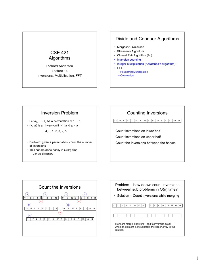
Divide and Conquer Algorithms Mergesort, Quicksort Strassens - PDF document

Divide and Conquer Algorithms • Mergesort, Quicksort • Strassen’s Algorithm CSE 421 • Closest Pair Algorithm (2d) Algorithms • Inversion counting • Integer Multiplication (Karatsuba’s Algorithm) Richard Anderson • FFT Lecture 14 – Polynomial Multiplication Inversions, Multiplication, FFT – Convolution Inversion Problem Counting Inversions • Let a 1 , . . . a n be a permutation of 1 . . n 11 12 4 1 7 2 3 15 9 5 16 8 6 13 10 14 • (a i , a j ) is an inversion if i < j and a i > a j Count inversions on lower half 4, 6, 1, 7, 3, 2, 5 Count inversions on upper half • Problem: given a permutation, count the number Count the inversions between the halves of inversions • This can be done easily in O(n 2 ) time – Can we do better? Problem – how do we count inversions Count the Inversions between sub problems in O(n) time? 4 2 3 1 • Solution – Count inversions while merging 11 12 4 1 7 2 3 15 9 5 16 8 6 13 10 14 8 6 14 10 1 2 3 4 7 11 12 15 5 6 8 9 10 13 14 16 11 12 4 1 7 2 3 15 9 5 16 8 6 13 10 14 19 43 11 12 4 1 7 2 3 15 9 5 16 8 6 13 10 14 Standard merge algorithm – add to inversion count when an element is moved from the upper array to the solution 1

Use the merge algorithm to count Inversions inversions • Counting inversions between two sorted lists 1 4 11 12 2 3 7 15 – O(1) per element to count inversions x x x x x x x x y y y y y y y y z z z z z z z z z z z z z z z z 5 8 9 16 6 10 13 14 • Algorithm summary – Satisfies the “Standard recurrence” – T(n) = 2 T(n/2) + cn Indicate the number of inversions for each element detected when merging Integer Arithmetic Recursive Algorithm (First attempt) x = x 1 2 n/2 + x 0 9715480283945084383094856701043643845790217965702956767 + 1242431098234099057329075097179898430928779579277597977 y = y 1 2 n/2 + y 0 xy = (x 1 2 n/2 + x 0 ) (y 1 2 n/2 + y 0 ) = x 1 y 1 2 n + (x 1 y 0 + x 0 y 1 )2 n/2 + x 0 y 0 Runtime for standard algorithm to add two n digit numbers: 2095067093034680994318596846868779409766717133476767930 Recurrence: X 5920175091777634709677679342929097012308956679993010921 Run time: Runtime for standard algorithm to multiply two n digit numbers: Simple algebra Karatsuba’s Algorithm x = x 1 2 n/2 + x 0 Multiply n-digit integers x and y y = y 1 2 n/2 + y 0 Let x = x 1 2 n/2 + x 0 and y = y 1 2 n/2 + y 0 Recursively compute xy = x 1 y 1 2 n + (x 1 y 0 + x 0 y 1 ) 2 n/2 + x 0 y 0 a = x 1 y 1 b = x 0 y 0 p = (x 1 + x 0 )(y 1 + y 0 ) Return a2 n + (p – a – b)2 n/2 + b p = (x 1 + x 0 )(y 1 + y 0 ) = x 1 y 1 + x 1 y 0 + x 0 y 1 + x 0 y 0 Recurrence: T(n) = 3T(n/2) + cn 2

FFT, Convolution and Polynomial Complex Analysis Multiplication • Polar coordinates: re θ i • Preview • e θ i = cos θ + i sin θ – FFT - O(n log n) algorithm • Evaluate a polynomial of degree n at n points in • A is a n th root of unity if a n = 1 O(n log n) time • Square roots of unity: +1, -1 – Computation of Convolution and Polynomial Multiplication (in O(n log n)) time • Fourth roots of unity: +1, -1, i, -i • Eighth roots of unity: +1, -1, i, -i, β + i β , β - i β , - β + i β , - β - i β where β = sqrt(2) e 2 π ki/n Convolution • e 2 π i = 1 • a 0 , a 1 , a 2 , . . ., a m-1 • e π i = -1 • b 0 , b 1 , b 2 , . . ., b n-1 • n th roots of unity: e 2 π ki/n for k = 0 …n-1 • c 0 , c 1 , c 2 , . . .,c m+n-2 where c k = Σ i+j=k a i b j • Notation: ω k,n = e 2 π ki/n • Interesting fact: 1 + ω k,n + ω 2k,n + ω 3k,n + . . . + ω n-1k,n = 0 for k != 0 Applications of Convolution FFT Overview • Polynomial Multiplication • Polynomial interpolation • Signal processing – Given n+1 points (x i ,y i ), there is a unique polynomial P of degree at most n which – Gaussian smoothing satisfies P(x i ) = y i – Sequence a 1 , a 2 , . . ., a n – Mask, w -k , w -(k-1) , . . ., w -1 , w 0 , w 1 , . . ., w k-1 , w k • Addition of random variables 3

Polynomial Multiplication FFT • Polynomial A(x) = a 0 + a 1 x + . . . + a n-1 x n-1 n-1 degree polynomials A(x) = a 0 + a 1 x + a 2 x 2 + … +a n-1 x n-1 , C(x) = A(x)B(x) • Compute A( ω j,n ) for j = 0, . . ., n-1 C(x)=c 0 +c 1 x + c 2 x 2 + … + c 2n-2 x 2n-2 B(x) = b 0 + b 1 x + b 2 x 2 + …+ b n-1 x n-1 p 1 , p 2 , . . ., p 2n A(p 1 ), A(p 2 ), . . ., A(p 2n ) C(p 1 ), C(p 2 ), . . ., C(p 2n ) B(p 1 ), B(p 2 ), . . ., B(p 2n ) C(p i ) = A(p i )B(p i ) 4