SLIDE 1 CS70: Lecture 37.
Markov Chains (contd.): First Passage Time: First Step Equations
- 1. Brief Recap of Markov Chains
- 2. First Passage Time – First Step Equations
- 3. Parting Thoughts
Brief Recap of Markov Chains
◮ Finite set X ;π0;P = {P(i,j),i,j ∈ X }; ◮ Pr[X0 = i] = π0(i),i ∈ X ◮ Pr[Xn+1 = j | X0,...,Xn = i] = P(i,j),i,j ∈ X ,n ≥ 0. ◮ Note: Pr[X0 = i0,X1 = i1,...,Xn = in] = π0(i0)P(i0,i1)···P(in−1,in). ◮ Irreducible MC: every state reachable from every other state ◮ State-transition equations: πm+1(j) = ∑i πm(i)P(i,j),∀j ∈ X . With
πm,πm+1 as row vectors, these identities are written as πm+1 = πmP.
◮ π1 = π0P,π2 = π1P = π0PP = π0P2,.... πn = π0Pn,n ≥ 0. ◮ Invariant Distribution: A distribution π0 is invariant iff π0P = π0.
These equations are called the balance equations.
◮ Finite irreducible Markov Chains have unique invariant
distribution.
◮ Balance Equations: Prob. Flow In = Prob. Flow out of every
state.
Balance Equations: 2-state MC example
πP = π ⇔ [π(1),π(2)]
a b 1−b
⇔ π(1)(1−a)+π(2)b = π(1) and π(1)a+π(2)(1−b) = π(2) ⇔ π(1)a = π(2)b.
- Prob. flow leaving state 1 = Prob. flow entering state 1
These equations are redundant! We have to add an equation: π(1)+π(2) = 1. Then we find π = [ b a+b, a a+b].
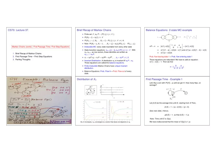
Distribution of Xn
1 0.8 1 2 3 0.7 0.3 0.6 0.4 0.2
1 2 3 n X
n
n
m m + 1 m m
πm(1) πm(2) πm(3) πm(1) πm(2) πm(3)
π0 = [0, 1, 0] π0 = [1, 0, 0]
As m increases, πm converges to a vector that does not depend on π0.
First Passage Time - Example 1
Let’s flip a coin with Pr[H] = p until we get H. How many flips, on average? Let β(S) be the average time until E, starting from S Then, β(S) = 1+(q ×β(S))+(p ×0). (See next slide.) Hence, pβ(S) = 1, so that β(S) = 1/p. Note: Time until E is G(p). We have rediscovered that the mean of G(p) is 1/p.
SLIDE 2 First Passage Time - Example 1
Let’s flip a coin with Pr[H] = p until we get H. Average no. of flips? Let β(S) be the average time until E. Then, β(S) = 1+(q ×β(S))+(p ×0). Justification: Let N be the random number of steps until E, starting from S. Let also N′ be the number of steps until E, after the second visit to S. Finally, let Z = 1{first flip = H} = 1 if first flip is H and 0 else. Then, N = 1+(1−Z)×N′ +Z ×0. Now, Z and N′ are independent. Also, E[N′] = E[N] = β(S). Hence, taking expectation of both sides of the equation, we get: β(S) = E[N] = 1+((1−p)×E[N′])+(p×0) = 1+(q ×β(S))+(p×0).
First Passage Time - Example 2
Let’s flip a coin with Pr[H] = p until we get two consecutive Hs. How many flips, on average? Here is a picture: Let β(i) be the average time from state i until the MC hits state E. We claim that (these are called the first step equations) β(S) = 1+pβ(H)+qβ(T) β(H) = 1+p0+qβ(T) β(T) = 1+pβ(H)+qβ(T). Solving, we find β(S) = 2+3qp−1 +q2p−2. (E.g., β(S) = 6 if p = 1/2.)
First Passage Time - Example 2
Let us justify the first step equation for β(T). The others are similar. Let N(T) be the random number of steps, starting from T until the MC hits E. Let also N(H) be defined similarly. Finally, let N′(T) be the number of steps after the second visit to T until the MC hits E. Then, N(T) = 1+Z ×N(H)+(1−Z)×N′(T) where Z = 1{first flip in T is H}. Since Z and N(H) are independent, and Z and N′(T) are independent, taking expectations, we get E[N(T)] = 1+pE[N(H)]+qE[N′(T)], i.e., β(T) = 1+pβ(H)+qβ(T).
First Passage Time - Example 3: Practice Exercise
You keep rolling a fair six-sided die until the sum of the last two rolls is 8. Question: How many times do you have to roll the die before you stop, on average? Spoiler Alert: Solution on next slide (but don’t look: try to do it yourself first!)
Example 3: Practice Exercise Solution
β(S) = 1+ 1 6
6
∑
j=1
β(j);β(1) = 1+ 1 6
6
∑
j=1
β(j);β(i) = 1+ 1 6
∑
j=1,...,6;j=8−i
β(j),i = 2,...,6. Symmetry: β(2) = ··· = β(6) =: γ. Also, β(1) = β(S). Thus, β(S) = 1+(5/6)γ +β(S)/6; γ = 1+(4/6)γ +(1/6)β(S). ⇒ ···β(S) = 8.4.
First Step Equations
Let Xn be a MC on X and A ⊂ X . Define TA = min{n ≥ 0 | Xn ∈ A}. Let β(i) = E[TA | X0 = i],i ∈ X . The FSE are β(i) = 0,i ∈ A β(i) = 1+∑
j
P(i,j)β(j),i / ∈ A
SLIDE 3 Summary
Markov Chains
◮ Markov Chain: Pr[Xn+1 = j|X0,...,Xn = i] = P(i,j) ◮ First Passage Time:
◮ A ⊂ X ;β(i) = E[TA|X0 = i]; ◮ β(i) = 1+∑j P(i,j)β(j);
◮ FSE: β(i) = 1+∑j P(i,j)β(j); ◮ πn = π0Pn ◮ π is invariant iff πP = π ◮ Irreducible ⇒ one and only one invariant distribution π
Probability part of the course: key takeaways?
What should I take away about probability from this course? I mean, after the final?
◮ Given the uncertainty around us, we should understand some
- probability. “Being precise about being imprecise.”
◮ 4 key concepts:
- 1. Learn from observations to revise our biases, given by the
role of the prior; Bayes’ Theorem;
- 2. Confidence Intervals: CLT, Cheybyshev Bounds, WLLN.
- 3. Regression/Estimation: L[Y|X],E[Y|X]
- 4. Markov Chains: Sequence of RVs, P[Xn+1 = xn+1|Xn =
xn,Xn−1 = xn−1,Xn−2 = xn−2,...] = P[Xn+1 = xn+1|Xn = xn], Balance Equations.
◮ Quantifying our degree of certainty. This clear thinking invites us
to question vague statements, and to convert them into precise ideas.
Random Thoughts Famous Quotes: French mathematician Pierre-Simon Laplace (Translated from French): “The theory of probabilities is basically just common sense reduced to calculus” Famous Quotes: Attributed by Mark Twain to British Prime Minister Benjamin Disraeli: ”There are three kinds of lies: lies, damned lies, and statistics.”
Confusing Statistics: Simpson’s Paradox
The numbers are applications and admissions of males and females to the two colleges of a university. Overall, the admission rate of male students is 80% whereas it is only 51% for female students. A closer look shows that the admission rate is larger for female students in both colleges.... Female students happen to apply more to the college that admits fewer students.
More on Confusing Statistics
Statistics are often confusing:
◮ The average household annual income in the US is $72k.
Yes, but the median is $52k.
◮ The false alarm rate for prostate cancer is only 1%. Great,
but only 1 person in 8,000 has that cancer. So, there are 80 false alarms for each actual case.
◮ The Texas sharpshooter fallacy. Look at people living close
to power lines. You find clusters of cancers. You will also find such clusters when looking at people eating kale.
◮ False causation. Vaccines cause autism. Both vaccination
and autism rates increased....
◮ Beware of statistics reported in the media!
Confirmation Bias
Confirmation bias is the tendency to search for, interpret, and recall information in a way that confirms one’s beliefs or hypotheses, while giving disproportionately less consideration to alternative possibilities. Confirmation biases contribute to overconfidence in personal beliefs and can maintain or strengthen beliefs in the face of contrary evidence. Three aspects:
◮ Biased search for information. E.g., ignoring articles that
dispute your beliefs.
◮ Biased interpretation. E.g., putting more weight on
confirmation than on contrary evidence.
◮ Biased memory. E.g., remembering facts that confirm your
beliefs and forgetting others.
SLIDE 4
Confirmation Bias: An experiment
There are two bags. One with 60% red balls and 40% blue balls; the other with the opposite fractions. One selects one of the two bags. As one draws balls one at time, one asks people to declare whether they think one draws from the first or second bag. Surprisingly, people tend to be reinforced in their original belief, even when the evidence accumulates against it.
Being Rational: ‘Thinking, Fast and Slow’
In this book, Daniel Kahneman discusses examples of our irrationality. Here are a few examples:
◮ A judge rolls a die in the morning. In the afternoon, he has to
sentence a criminal. Statistically, the sentence tends to be heavier if the outcome of the morning roll was high.
◮ People tend to be more convinced by articles printed in Times
Roman instead of Computer Modern Sans Serif.
◮ Perception illusions: Which horizontal line is longer?
It is difficult to think clearly!
What’s Next?
Professors, I loved this course so much! I want to learn more about discrete math and probability! Funny you should ask! How about
◮ CS170: Efficient Algorithms and Intractable Problems a.k.a.
Introduction to CS Theory: Graphs, Dynamic Programming, Complexity.
◮ EECS126: Probability in EECS: An Applications-Driven Course:
PageRank, Digital Links, Tracking, Speech Recognition, Planning, etc. Hands on labs with python experiments (GPS, Auctions, Kalman Filtering, RNA sequencing, ...).
◮ CS188: Artificial Intelligence: Hidden Markov Chains, Bayes Networks,
Neural Networks.
◮ CS189: Introduction to Machine Learning: Regression, Neural
Networks, Learning, etc. Programming experiments with real-world applications.
Parting Thoughts
You have worked hard and learned a lot in this course! Proofs, Graphs, Stable Marriage, Mod(p), RSA, Reed-Solomon, Decidability, Probability, ... , HW option or Test-only option? how to handle stress, how to sleep less, how to keep smiling, ... Difficult course? Yes! Useful? You bet! Finally, THANK YOU on behalf of Prof. Rao and me for persevering through this course! It has been an absolute pleasure! Let us also not forget to thank the dedicated EECS70 Staff:
◮ The Thrilling TAs ◮ The Terrific Tutors ◮ The Rigorous Readers ◮ The Amazing Assistants
GOOD LUCK IN YOUR FINAL EXAM!!!