CS475/CM375 Lecture 4: Sept 22 Sparse Gaussian Elimination, Graph - PDF document

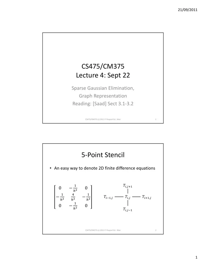
21/09/2011 CS475/CM375 Lecture 4: Sept 22 Sparse Gaussian Elimination, Graph Representation Reading: [Saad] Sect 3.1 ‐ 3.2 CS475/CM375 (c) 2011 P. Poupart & J. Wan 1 5 ‐ Point Stencil • An easy way to denote 2D finite difference equations � �,��� � 0 � 0 � � � � � � � � ���,� � �,� � ���,� � � � � � � � 0 � 0 � � � �,��� CS475/CM375 (c) 2011 P. Poupart & J. Wan 2 1

21/09/2011 Numbering of unknowns • Picture: • Note: the values on the boundary are zero � � �,� ⋯ � �,� �,� � � �,� ⋯ � �,� �,� • The unknowns are: ⋮ ⋮ ⋱ ⋮ � � �,� ⋯ � �,� �,� • Total number � � � � � � � ≡ � CS475/CM375 (c) 2011 P. Poupart & J. Wan 3 Natural ordering • Ordering: first in the x ‐ direction, then y ‐ direction – i.e., � �,� , � �,� , … , � �,� ; � �,� , � �,� , … • The system of linear equations � � � � � 1, � � 1: � � � �,� � � � � �,� � � � � �,� � � �,� � � � � � � 2, � � 1: � � � � �,� � � � � �,� � � � � �,� � � � � �,� � � �,� ⋮ � � � � � �, � � �: � � � � �,��� � � � � ���,� � � � � �,� � � �,� CS475/CM375 (c) 2011 P. Poupart & J. Wan 4 2

21/09/2011 Matrix Form • Example �� � 4, � � 16� CS475/CM375 (c) 2011 P. Poupart & J. Wan 5 Graph Representation of Matrices • Given a sparse matrix � , a node is associated with each row. • If � �,� � 0 , there exists an edge from node � to � 1 � � 2 � � � � � � : � � � 3 4 � � CS475/CM375 (c) 2011 P. Poupart & J. Wan 6 3

21/09/2011 Graph for Symmetric Matrices • For symmetric matrices, arrows can be dropped (as well as self loops) 1 � � � � � � 2 � � � � : 3 � � � 4 � � � CS475/CM375 (c) 2011 P. Poupart & J. Wan 7 Physical/Geometric Interpretation • Graph of a matrix often has a simple physical/geometric interpretation – 1D Laplacian � � � � : – 2D Laplacian � � � � : CS475/CM375 (c) 2011 P. Poupart & J. Wan 8 4

21/09/2011 GE and Matrix Graph • “Visualize” eliminations by matrix graph � � � � � � � � � 0 � � ∎ GE e.g . � � � � � � � � 0 ∎ � � fill ‐ in � � : CS475/CM375 (c) 2011 P. Poupart & J. Wan 9 GE and Matrix Graph • Elimination of node � produces a new graph with – Node � deleted, all edges containing node � deleted – New edge ��, �� added (fill ‐ in) if there was an edge ��, �� & ��, �� in the old graph. • Notes – Matrix (with symmetric structure) graph is unchanged by renumbering of the nodes – But orderings (which nodes to be removed first) may result in much less fill during GE. CS475/CM375 (c) 2011 P. Poupart & J. Wan 10 5

21/09/2011 Ordering Algorithms • Consider the following matrix graph: � � � � • Assume � � ≫ � � . If we use the natural ordering, what would the matrix look like? CS475/CM375 (c) 2011 P. Poupart & J. Wan 11 Ordering Algorithms • If we had numbered along y ‐ direction first, the matrix becomes: • Which ordering results in less fill? Why? CS475/CM375 (c) 2011 P. Poupart & J. Wan 12 6

21/09/2011 Band Matrices • Note: GE preserves band structure – Picture: • Amount of work to factor a band matrix: – ��� � �� where � � bandwidth � � – x ‐ first ordering → ����� �� � � � � � �� – y ‐ first ordering → ����� �� � ��� � CS475/CM375 (c) 2011 P. Poupart & J. Wan 13 Envelope Methods • In general, bandwidth is not the same for each row – Example: • In each row, fill can occur only between the 1 st nonzero entry and the diagonal. • To limit the amount of fill, keep the envelope as close to the diagonal as possible CS475/CM375 (c) 2011 P. Poupart & J. Wan 14 7

21/09/2011 Envelope Methods • Try to number nodes so that graph neighbours have numbers as close together as possible – Example: CS475/CM375 (c) 2011 P. Poupart & J. Wan 15 8