
Utah School of Computing Spring 2013 Computer Graphics CS5600
Spring 2013 Utah School of Computing 1
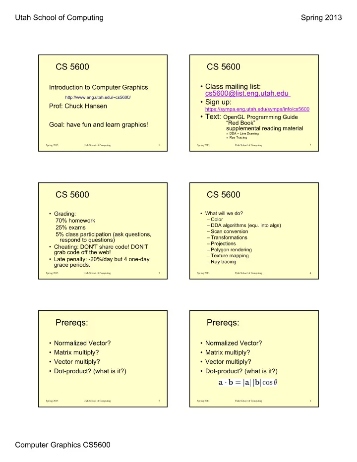
CS 5600
Introduction to Computer Graphics Prof: Chuck Hansen Goal: have fun and learn graphics!
http://www.eng.utah.edu/~cs5600/
Spring 2013 Utah School of Computing 2
CS 5600
- Class mailing list:
cs5600@list.eng.utah.edu
- Sign up:
https://sympa.eng.utah.edu/sympa/info/cs5600
- Text: OpenGL Programming Guide
“Red Book” supplemental reading material
» DDA – Line Drawing » Ray Tracing
Spring 2013 Utah School of Computing 3
CS 5600
- Grading:
70% homework 25% exams 5% class participation (ask questions, respond to questions)
- Cheating: DON'T share code! DON'T
grab code off the web!
- Late penalty: -20%/day but 4 one-day
grace periods.
Spring 2013 Utah School of Computing 4
CS 5600
- What will we do?
– Color – DDA algorithms (equ. into algs) – Scan conversion – Transformations – Projections – Polygon rendering – Texture mapping – Ray tracing
Spring 2013 Utah School of Computing 5
Prereqs:
- Normalized Vector?
- Matrix multiply?
- Vector multiply?
- Dot-product? (what is it?)
Spring 2013 Utah School of Computing 6
Prereqs:
- Normalized Vector?
- Matrix multiply?
- Vector multiply?
- Dot-product? (what is it?)