CS 188: Artificial Intelligence Review of Probability, Bayes nets - - PDF document

1

CS 188: Artificial Intelligence

Review of Probability, Bayes’ nets

DISCLAIMER: It is insufficient to simply study these slides, they are merely meant as a quick refresher of the high-level ideas covered. You need to study all materials covered in lecture, section, assignments and projects ! Pieter Abbeel – UC Berkeley Many slides adapted from Dan Klein

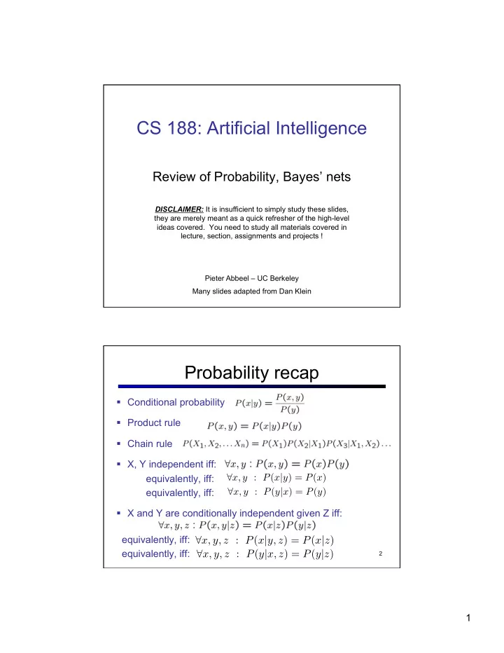
Probability recap

§ Conditional probability § Product rule § Chain rule § X, Y independent iff: equivalently, iff: equivalently, iff: § X and Y are conditionally independent given Z iff: equivalently, iff: equivalently, iff:

2

∀x, y : P(x|y) = P(x)

∀x, y, z : P(x|y, z) = P(x|z) ∀x, y, z : P(y|x, z) = P(y|z)

∀x, y : P(y|x) = P(y)

2

Inference by Enumeration

§ P(sun)? § P(sun | winter)? § P(sun | winter, hot)?

S T W P summer hot sun 0.30 summer hot rain 0.05 summer cold sun 0.10 summer cold rain 0.05 winter hot sun 0.10 winter hot rain 0.05 winter cold sun 0.15 winter cold rain 0.20

3

Bayes’ Nets Recap

§ Representation

§ Chain rule -> Bayes’ net = DAG + CPTs

§ Conditional Independences

§ D-separation

§ Probabilistic Inference

§ Enumeration (exact, exponential complexity) § Variable elimination (exact, worst-case exponential complexity, often better) § Probabilistic inference is NP-complete § Sampling (approximate)

4

3

Chain Rule à Bayes net

§ Chain rule: can always write any joint distribution as an incremental product of conditional distributions

§ Bayes nets: make conditional independence assumptions of the form: giving us:

5

P(xi|x1 · · · xi−1) = P(xi|parents(Xi))

B E A J M

Probabilities in BNs

§ Bayes’ nets implicitly encode joint distributions

§ As a product of local conditional distributions § To see what probability a BN gives to a full assignment, multiply all the relevant conditionals together: § Example:

§ This lets us reconstruct any entry of the full joint § Not every BN can represent every joint distribution

§ The topology enforces certain conditional independencies

6

4

Example: Alarm Network

Burglary Earthqk Alarm John calls Mary calls B P(B) +b 0.001 ¬b 0.999 E P(E) +e 0.002 ¬e 0.998 B E A P(A|B,E) +b +e +a 0.95 +b +e ¬a 0.05 +b ¬e +a 0.94 +b ¬e ¬a 0.06 ¬b +e +a 0.29 ¬b +e ¬a 0.71 ¬b ¬e +a 0.001 ¬b ¬e ¬a 0.999 A J P(J|A) +a +j 0.9 +a ¬j 0.1 ¬a +j 0.05 ¬a ¬j 0.95 A M P(M|A) +a +m 0.7 +a ¬m 0.3 ¬a +m 0.01 ¬a ¬m 0.99

Size of a Bayes’ Net for

§ How big is a joint distribution over N Boolean variables?

2N

§ Size of representation if we use the chain rule

2N

§ How big is an N-node net if nodes have up to k parents?

O(N * 2k+1)

§ Both give you the power to calculate § BNs:

§ Huge space savings! § Easier to elicit local CPTs § Faster to answer queries

8

5

Bayes Nets: Assumptions

§ Assumptions made by specifying the graph: § Given a Bayes net graph additional conditional independences can be read off directly from the graph

§ Question: Are two nodes guaranteed to be independent given certain evidence? § If no, can prove with a counter example

§ I.e., pick a set of CPT’s, and show that the independence assumption is violated by the resulting distribution

§ If yes, can prove with

§ Algebra (tedious)

§ D-separation (analyzes graph)

9

P(xi|x1 · · · xi−1) = P(xi|parents(Xi))

D-Separation

§ Question: Are X and Y conditionally independent given evidence vars {Z}?

§ Yes, if X and Y “separated” by Z § Consider all (undirected) paths from X to Y § No active paths = independence!

§ A path is active if each triple is active:

§ Causal chain A → B → C where B is unobserved (either direction) § Common cause A ← B → C where B is unobserved § Common effect (aka v-structure) A → B ← C where B or one of its descendents is observed

§ All it takes to block a path is a single inactive segment

Active Triples Inactive Triples

6

D-Separation

§ Given query § Shade all evidence nodes § For all (undirected!) paths between and

§ Check whether path is active

§ If active return

§ (If reaching this point all paths have been checked and shown inactive)

§ Return

11

Xi ⊥ ⊥ Xj|{Xk1, ..., Xkn}

Xi ⊥ ⊥ Xj|{Xk1, ..., Xkn}

? Xi ⊥ ⊥ Xj|{Xk1, ..., Xkn}

Example

R T B D L T’ Yes Yes Yes

12

7

All Conditional Independences

§ Given a Bayes net structure, can run d- separation to build a complete list of conditional independences that are necessarily true of the form § This list determines the set of probability distributions that can be represented by Bayes’ nets with this graph structure

13

Xi ⊥ ⊥ Xj|{Xk1, ..., Xkn}

Topology Limits Distributions

§ Given some graph topology G, only certain joint distributions can be encoded § The graph structure guarantees certain (conditional) independences § (There might be more independence) § Adding arcs increases the set of distributions, but has several costs § Full conditioning can encode any distribution X Y Z X Y Z X Y Z

14

X Y Z X Y Z X Y Z X Y Z X Y Z X Y Z X Y Z

{X ⊥ ⊥ Z | Y }

{X ⊥ ⊥ Y, X ⊥ ⊥ Z, Y ⊥ ⊥ Z, X ⊥ ⊥ Z | Y, X ⊥ ⊥ Y | Z, Y ⊥ ⊥ Z | X}

{}

8

Inference by Enumeration

§ Given unlimited time, inference in BNs is easy § Recipe:

§ State the marginal probabilities you need § Figure out ALL the atomic probabilities you need § Calculate and combine them

§ Example:

15

B E A J M

Example: Enumeration

§ In this simple method, we only need the BN to synthesize the joint entries

16

9

Variable Elimination

§ Why is inference by enumeration so slow?

§ You join up the whole joint distribution before you sum

• ut the hidden variables

§ You end up repeating a lot of work!

§ Idea: interleave joining and marginalizing!

§ Called “Variable Elimination” § Still NP-hard, but usually much faster than inference by enumeration

17

§ Track objects called factors § Initial factors are local CPTs (one per node) § Any known values are selected

§ E.g. if we know , the initial factors are

§ VE: Alternately join factors and eliminate variables

18

Variable Elimination Outline

+r ¡ 0.1 ¡

• ­‑r ¡

0.9 ¡ +r ¡ +t ¡ 0.8 ¡ +r ¡

• ­‑t ¡

0.2 ¡

• ­‑r ¡

+t ¡ 0.1 ¡

• ­‑r ¡
• ­‑t ¡

0.9 ¡ +t ¡ +l ¡ 0.3 ¡ +t ¡

• ­‑l ¡

0.7 ¡

• ­‑t ¡

+l ¡ 0.1 ¡

• ­‑t ¡
• ­‑l ¡

0.9 ¡ +t ¡ +l ¡ 0.3 ¡

• ­‑t ¡

+l ¡ 0.1 ¡ +r ¡ 0.1 ¡

• ­‑r ¡

0.9 ¡ +r ¡ +t ¡ 0.8 ¡ +r ¡

• ­‑t ¡

0.2 ¡

• ­‑r ¡

+t ¡ 0.1 ¡

• ­‑r ¡
• ­‑t ¡

0.9 ¡

T R L

10

Variable Elimination Example

19

Sum out R

T L

+r ¡ +t ¡ 0.08 ¡ +r ¡

• ­‑t ¡

0.02 ¡

• ­‑r ¡

+t ¡ 0.09 ¡

• ­‑r ¡
• ­‑t ¡

0.81 ¡ +t ¡ +l ¡ 0.3 ¡ +t ¡ -­‑l ¡ 0.7 ¡

• ­‑t ¡ +l ¡ 0.1 ¡
• ­‑t ¡
• ­‑l ¡ 0.9 ¡

+t ¡ 0.17 ¡

• ­‑t ¡

0.83 ¡ +t ¡ +l ¡ 0.3 ¡ +t ¡ -­‑l ¡ 0.7 ¡

• ­‑t ¡ +l ¡ 0.1 ¡
• ­‑t ¡
• ­‑l ¡ 0.9 ¡

T R L

+r ¡ 0.1 ¡

• ­‑r ¡

0.9 ¡ +r ¡ +t ¡ 0.8 ¡ +r ¡ -­‑t ¡ 0.2 ¡

• ­‑r ¡ +t ¡ 0.1 ¡
• ­‑r ¡
• ­‑t ¡ 0.9 ¡

+t ¡ +l ¡ 0.3 ¡ +t ¡ -­‑l ¡ 0.7 ¡

• ­‑t ¡ +l ¡ 0.1 ¡
• ­‑t ¡
• ­‑l ¡ 0.9 ¡

Join R

R, T L

Variable Elimination Example

Join T Sum out T

T, L L

* VE is variable elimination

T L

+t ¡ 0.17 ¡

• ­‑t ¡

0.83 ¡ +t ¡ +l ¡ 0.3 ¡ +t ¡ -­‑l ¡ 0.7 ¡

• ­‑t ¡ +l ¡ 0.1 ¡
• ­‑t ¡
• ­‑l ¡ 0.9 ¡

+t ¡ +l ¡ 0.051 ¡ +t ¡ -­‑l ¡

0.119 ¡

• ­‑t ¡ +l ¡ 0.083 ¡
• ­‑t ¡
• ­‑l ¡

0.747 ¡

+l ¡ 0.134 ¡

• ­‑l ¡

0.886 ¡

11

Example

Choose A

21

Example

Choose E Finish with B

Normalize

22

12

General Variable Elimination

§ Query: § Start with initial factors:

§ Local CPTs (but instantiated by evidence)

§ While there are still hidden variables (not Q or evidence):

§ Pick a hidden variable H § Join all factors mentioning H § Eliminate (sum out) H

§ Join all remaining factors and normalize

23

Another (bit more abstractly worked

• ut) Variable Elimination Example

24

Computational complexity critically depends on the largest factor being generated in this process. Size of factor = number of entries in table. In example above (assuming binary) all factors generated are of size 2 --- as they all only have one variable (Z, Z, and X3 respectively).

13

§ For the query P(Xn|y1,…,yn) work through the following two different

• rderings as done in previous slide: Z, X1, …, Xn-1 and X1, …, Xn-1,
• Z. What is the size of the maximum factor generated for each of the
• rderings?

§ Answer: 2n versus 2 (assuming binary) § In general: the ordering can greatly affect efficiency.

Variable Elimination Ordering

25

… …

Computational and Space Complexity of Variable Elimination

§ The computational and space complexity of variable elimination is determined by the largest factor § The elimination ordering can greatly affect the size of the largest factor.

§ E.g., previous slide’s example 2n vs. 2

§ Does there always exist an ordering that only results in small factors?

§ No!

26

14

Worst Case Complexity?

§ Consider the 3-SAT clause: which can be encoded by the following Bayes’ net: § If we can answer P(z) equal to zero or not, we answered whether the 3-SAT problem has a solution. § Subtlety: why the cascaded version of the AND rather than feeding all OR clauses into a single AND? Answer: a single AND would have an exponentially large CPT, whereas with representation above the Bayes’ net has small CPTs only. § Hence inference in Bayes’ nets is NP-hard. No known efficient probabilistic inference in general. 27

… …

Polytrees

§ A polytree is a directed graph with no undirected cycles § For poly-trees you can always find an

• rdering that is efficient

§ Try it!!

§ Cut-set conditioning for Bayes’ net inference

§ Choose set of variables such that if removed

• nly a polytree remains

§ Think about how the specifics would work out!

28

15

Approximate Inference: Sampling

§ Basic idea:

§ Draw N samples from a sampling distribution S § Compute an approximate posterior probability § Show this converges to the true probability P

§ Why? Faster than computing the exact answer § Prior sampling:

§ Sample ALL variables in topological order as this can be done quickly

§ Rejection sampling for query

§ = like prior sampling, but reject when a variable is sampled inconsistent with the query, in this case when a variable Ei is sampled differently from ei

§ Likelihood weighting for query

§ = like prior sampling but variables Ei are not sampled, when it’s their turn, they get set to ei, and the sample gets weighted by P(ei | value of parents(ei) in current sample) § Gibbs sampling: repeatedly samples each non-evidence variable conditioned on all other variables à can incorporate downstream evidence

29

Prior Sampling

Cloudy Sprinkler Rain WetGrass Cloudy Sprinkler Rain WetGrass

30

+c ¡ 0.5 ¡

• ­‑c ¡

0.5 ¡ +c ¡ ¡ +s ¡ 0.1 ¡

• ­‑s ¡

0.9 ¡

• ­‑c ¡

¡ +s ¡ 0.5 ¡

• ­‑s ¡

0.5 ¡ +c ¡ ¡ +r ¡ 0.8 ¡

• ­‑r ¡

0.2 ¡

• ­‑c ¡

¡ +r ¡ 0.2 ¡

• ­‑r ¡

0.8 ¡ +s ¡ ¡ ¡ ¡ +r ¡ ¡ +w ¡ 0.99 ¡

• ­‑w ¡

0.01 ¡

• ­‑r ¡

¡ +w ¡ 0.90 ¡

• ­‑w ¡

0.10 ¡

• ­‑s ¡

¡ ¡ ¡ +r ¡ ¡ +w ¡ 0.90 ¡

• ­‑w ¡

0.10 ¡

• ­‑r ¡

¡ +w ¡ 0.01 ¡

• ­‑w ¡

0.99 ¡

Samples: +c, -s, +r, +w

• c, +s, -r, +w

…

16

Example

§ We’ll get a bunch of samples from the BN:

+c, -s, +r, +w +c, +s, +r, +w

• c, +s, +r, -w

+c, -s, +r, +w

• c, -s, -r, +w

§ If we want to know P(W)

§ We have counts <+w:4, -w:1> § Normalize to get P(W) = <+w:0.8, -w:0.2> § This will get closer to the true distribution with more samples § Can estimate anything else, too § What about P(C| +w)? P(C| +r, +w)? P(C| -r, -w)? § Fast: can use fewer samples if less time

Cloudy Sprinkler Rain WetGrass C S R W

31

Likelihood Weighting

32

+c ¡ 0.5 ¡

• ­‑c ¡

0.5 ¡ +c ¡ ¡ +s ¡ 0.1 ¡

• ­‑s ¡

0.9 ¡

• ­‑c ¡

¡ +s ¡ 0.5 ¡

• ­‑s ¡

0.5 ¡ +c ¡ ¡ +r ¡ 0.8 ¡

• ­‑r ¡

0.2 ¡

• ­‑c ¡

¡ +r ¡ 0.2 ¡

• ­‑r ¡

0.8 ¡ +s ¡ ¡ ¡ ¡ +r ¡ ¡ +w ¡ 0.99 ¡

• ­‑w ¡

0.01 ¡

• ­‑r ¡

¡ +w ¡ 0.90 ¡

• ­‑w ¡

0.10 ¡

• ­‑s ¡

¡ ¡ ¡ +r ¡ ¡ +w ¡ 0.90 ¡

• ­‑w ¡

0.10 ¡

• ­‑r ¡

¡ +w ¡ 0.01 ¡

• ­‑w ¡

0.99 ¡

Samples: +c, +s, +r, +w … Cloudy Sprinkler Rain WetGrass Cloudy Sprinkler Rain WetGrass

17

Likelihood Weighting

§ Sampling distribution if z sampled and e fixed evidence § Now, samples have weights § Together, weighted sampling distribution is consistent

Cloudy R C S W

33

Gibbs Sampling

§ Idea: instead of sampling from scratch, create samples that are each like the last one. § Procedure: resample one variable at a time, conditioned

• n all the rest, but keep evidence fixed.

§ Properties: Now samples are not independent (in fact they’re nearly identical), but sample averages are still consistent estimators! § What’s the point: both upstream and downstream variables condition on evidence.

34

18

Markov Models

§ A Markov model is a chain-structured BN

§ Each node is identically distributed (stationarity) § Value of X at a given time is called the state § As a BN:

§ The chain is just a (growing) BN

§ We can always use generic BN reasoning on it if we truncate the chain at a fixed length

§ Stationary distributions

§ For most chains, the distribution we end up in is independent of the initial distribution § Called the stationary distribution of the chain

§ Example applications: Web link analysis (Page Rank) and Gibbs Sampling

X2 X1 X3 X4

Hidden Markov Models

§ Underlying Markov chain over states S § You observe outputs (effects) at each time step § Speech recognition HMMs:

§ Xi: specific positions in specific words; Ei: acoustic signals

§ Machine translation HMMs:

§ Xi: translation options; Ei: Observations are words

§ Robot tracking:

§ Xi: positions on a map; Ei: range readings

X5 X2 E1 X1 X3 X4 E2 E3 E4 E5

19

Online Belief Updates

§ Every time step, we start with current P(X | evidence) § We update for time: § We update for evidence: § The forward algorithm does both at once (and doesn’t normalize)

X2 X1 X2 E2

Recap: Particle Filtering

§ Particles: track samples of states rather than an explicit distribution

38

Particles: (3,3) (2,3) (3,3) (3,2) (3,3) (3,2) (1,2) (3,3) (3,3) (2,3)

Elapse Weight Resample

Particles: (3,2) (2,3) (3,2) (3,1) (3,3) (3,2) (1,3) (2,3) (3,2) (2,2) Particles: (3,2) w=.9 (2,3) w=.2 (3,2) w=.9 (3,1) w=.4 (3,3) w=.4 (3,2) w=.9 (1,3) w=.1 (2,3) w=.2 (3,2) w=.9 (2,2) w=.4 (New) Particles: (3,2) (2,2) (3,2) (2,3) (3,3) (3,2) (1,3) (2,3) (3,2) (3,2)

20

Dynamic Bayes Nets (DBNs)

§ We want to track multiple variables over time, using multiple sources of evidence § Idea: Repeat a fixed Bayes net structure at each time § Variables from time t can condition on those from t-1 § Discrete valued dynamic Bayes nets are also HMMs

G1

a

E1a E1b G1

b

G2

a

E2a E2b G2

b

t =1 t =2 G3

a

E3a E3b G3

b

t =3

Best Explanation Queries

§ Query: most likely seq:

X5 X2 E1 X1 X3 X4 E2 E3 E4 E5

40

21

Best Explanation Query Solution Method 1: Search

§ States: {(), +x1, -x1, +x2, -x2, …, +xt, -xt} § Start state: () § Actions: in state xk, choose any assignment for state xk+1 § Cost: § Goal test: goal(xk) = true iff k == t

à Can run uniform cost graph search to find solution à Uniform cost graph search will take O( t d2 ). Think about this!

slight abuse of notation, assuming P(x1|x0) = P(x1)

Best Explanation Query Solution Method 2: Viterbi Algorithm (= max-product version of forward algorithm)

42

Viterbi computational complexity: O(t d2) Compare to forward algorithm:

22

Parameter Estimation

§ Estimating distribution of random variables like X or X | Y § Empirically: use training data

§ For each outcome x, look at the empirical rate of that value: § This is the estimate that maximizes the likelihood of the data

§ Laplace smoothing

§ Pretend saw every outcome k extra times § Smooth each condition independently:

r g g

Decision Networks

§ MEU: choose the action which maximizes the expected utility given the evidence § Can directly operationalize this with decision networks

§ Bayes nets with nodes for utility and actions § Lets us calculate the expected utility for each action

§ New node types:

§ Chance nodes (just like BNs) § Actions (rectangles, cannot have parents, act as observed evidence) § Utility node (diamond, depends

• n action and chance nodes)

Weather Forecast Umbrella U

44

23

Decision Networks

§ Action selection:

§ Instantiate all evidence § Set action node(s) each possible way § Calculate posterior for all parents of utility node, given the evidence § Calculate expected utility for each action § Choose maximizing action

Weather Forecast Umbrella U

45

Example: Decision Networks

Weather Umbrella U

W P(W) sun 0.7 rain 0.3 A W U(A,W) leave sun 100 leave rain take sun 20 take rain 70

Umbrella = leave Umbrella = take Optimal decision = leave

24

Example: Decision Networks

Weather Forecast =bad Umbrella U

A W U(A,W) leave sun 100 leave rain take sun 20 take rain 70 W P(W|F=bad) sun 0.34 rain 0.66

Umbrella = leave Umbrella = take Optimal decision = take

47

Decisions as Outcome Trees

48

U(t,s) W | {b} W | {b} t a k e leave sun U(t,r) rain U(l,s) U(l,r) rain sun {b}

25

VPI Example: Weather

Weather Forecast Umbrella U

A W U leave sun 100 leave rain take sun 20 take rain 70

MEU with no evidence MEU if forecast is bad MEU if forecast is good

F P(F) good 0.59 bad 0.41

Forecast distribution

49

Value of Information

§ Assume we have evidence E=e. Value if we act now: § Assume we see that E’ = e’. Value if we act then: § BUT E’ is a random variable whose value is unknown, so we don’t know what e’ will be § Expected value if E’ is revealed and then we act: § Value of information: how much MEU goes up by revealing E’ first then acting, over acting now: P(s | +e) {+e} a U {+e, +e’} a P(s | +e, +e’) U {+e} P(+e’ | +e)

{+e, +e’}

P(-e’ | +e)

{+e, +e’}

a

26

Example: Ghostbusters

§ In (static) Ghostbusters:

§ Belief state determined by evidence to date {e} § Tree really over evidence sets § Probabilistic reasoning needed to predict new evidence given past evidence

§ Solving POMDPs

§ One way: use truncated expectimax to compute approximate value of actions § What if you only considered busting or one sense followed by a bust? § You get a VPI-based agent!

a {e} e, a e’ {e, e’} a b b, a

• b

’ abust {e} {e}, asense e’ {e, e’} asense U(abust, {e}) abust U(abust, {e, e’})

51