CS 188: Artificial Intelligence Lecture 18: Speech Pieter Abbeel - PDF document

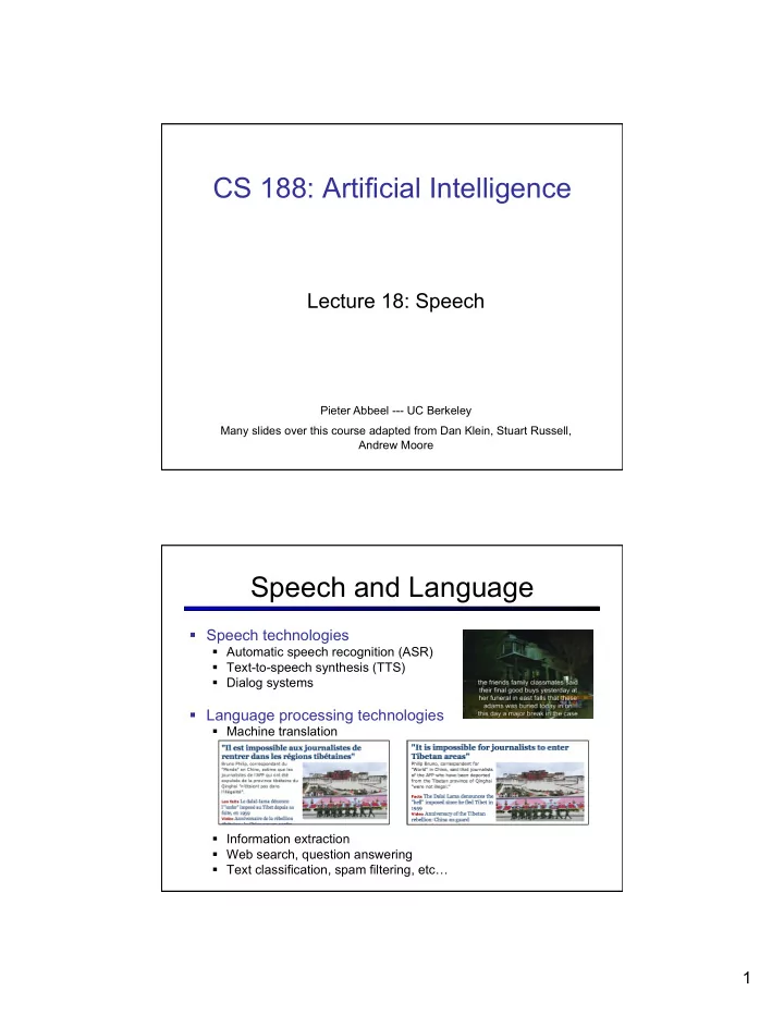
CS 188: Artificial Intelligence Lecture 18: Speech Pieter Abbeel --- UC Berkeley Many slides over this course adapted from Dan Klein, Stuart Russell, Andrew Moore Speech and Language § Speech technologies § Automatic speech recognition (ASR) § Text-to-speech synthesis (TTS) § Dialog systems § Language processing technologies § Machine translation § Information extraction § Web search, question answering § Text classification, spam filtering, etc … 1

Digitizing Speech 3 Speech in an Hour § Speech input is an acoustic wave form s p ee ch l a b “ l ” to “ a ” transition: Graphs from Simon Arnfield ’ s web tutorial on speech, 4 Sheffield: http://www.psyc.leeds.ac.uk/research/cogn/speech/tutorial/ 2

Spectral Analysis § Frequency gives pitch; amplitude gives volume § sampling at ~8 kHz phone, ~16 kHz mic (kHz=1000 cycles/sec) s p ee ch l a b amplitude § Fourier transform of wave displayed as a spectrogram § darkness indicates energy at each frequency frequency 5 Part of [ae] from “ lab ” § Complex wave repeating nine times § Plus smaller wave that repeats 4x for every large cycle § Large wave: freq of 250 Hz (9 times in .036 seconds) § Small wave roughly 4 times this, or roughly 1000 Hz [ demo ] 6 3

Resonances of the vocal tract § The human vocal tract as an open tube Closed end Open end Length 17.5 cm. § Air in a tube of a given length will tend to vibrate at resonance frequency of tube. § Constraint: Pressure differential should be maximal at (closed) glottal end and minimal at (open) lip end. 7 Figure from W. Barry Speech Science slides [ demo ] From Mark Liberman ’ s 8 website 4

Vowel [i] sung at successively higher pitches F#2 A2 C3 F#3 A3 C4 (middle C) A4 Figures from Ratree Wayland Acoustic Feature Sequence § Time slices are translated into acoustic feature vectors (~39 real numbers per slice) frequency …………………………………………… .. e 12 e 13 e 14 e 15 e 16 ……… .. § These are the observations, now we need the hidden states X 10 5

State Space § P(E|X) encodes which acoustic vectors are appropriate for each phoneme (each kind of sound) § P(X|X ’ ) encodes how sounds can be strung together § We will have one state for each sound in each word § From some state x, can only: § Stay in the same state (e.g. speaking slowly) § Move to the next position in the word § At the end of the word, move to the start of the next word § We build a little state graph for each word and chain them together to form our state space X 11 HMMs for Speech 12 6

Transitions with Bigrams 198015222 the first Training Counts 194623024 the same 168504105 the following 158562063 the world … 14112454 the door ----------------- 23135851162 the * Figure from Huang et al page 618 Decoding § While there are some practical issues, finding the words given the acoustics is an HMM inference problem § We want to know which state sequence x 1:T is most likely given the evidence e 1:T : § From the sequence x, we can simply read off the words 14 7