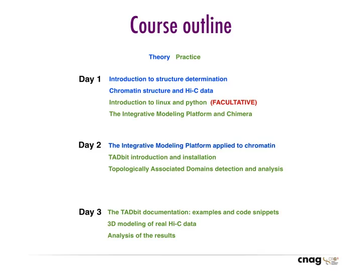
Course outline Theory Practice Day 1 Introduction to structure - - PowerPoint PPT Presentation

SLIDE 1

Course outline

Introduction to structure determination Chromatin structure and Hi-C data Introduction to linux and python (FACULTATIVE) The Integrative Modeling Platform and Chimera

Day 1

The Integrative Modeling Platform applied to chromatin TADbit introduction and installation Topologically Associated Domains detection and analysis

Day 2

The TADbit documentation: examples and code snippets 3D modeling of real Hi-C data Analysis of the results

Day 3

Theory Practice

SLIDE 2

3D structure determination

Davide Baù & François Serra

Genome Biology Group (CNAG) Structural Genomics Group (CRG)

SLIDE 3

Structural Genomics Group

http://www.marciuslab.org

SLIDE 4

Data groups

Laws of physics Statistical rules Experimental

• bservations

SLIDE 5

The importance of the 3D structure

The biochemical function of a molecule is defined by its interactions The 3D structure is more informative than sequence alone Evolution tends to conserve function and function depends more directly on structure than on sequence The biological function is in large part a consequence

• f these interations

SLIDE 6

Structure prediction vs determination

Experimental data inferred data X-Ray NMR Comparative Modeling Threading Ab-initio

SLIDE 7

Data integration

SLIDE 8

SLIDE 9

The four stages of integrative modeling

Stage 4: Analyzing Resulting Models and Information

Cluster 1 500 nm 180o Cluster 2 500 nm 180o Cluster 3 500 nm 180o Cluster 4 500 nm 180o

Stage 1: Gathering experimental and statistical Information Stage 2: Choosing How To Represent And Evaluate Models Stage 3: Finding Models That Score Well

SLIDE 10

Advantages of integrative modeling

Russel, D., Lasker, K., Webb, B., Velázquez-Muriel, J., Tjioe, E., Schneidman-Duhovny, D., Peterson, B., et al. (2012). PLoS Biology, 10(1), e1001244

• It facilitates the use of new information
• It maximizes accuracy, precision and completeness of the models
• It facilitates assessing the input information and output models
• It helps in understanding and assessing experimental accuracy

SLIDE 11

f(·)

Experiments Computations Physics Evolution

Integrative Modeling Platform

http://www.integrativemodeling.org

From: Russel, D. et al. PLOS Biology 10, e1001244 (2012).

SLIDE 12

Energy landscape

1 3 2

Local minima Global minimum

Energetically cheap

SLIDE 13

Energy landscape

1 3 2 Local minima Global minimum Energetically expensive

SLIDE 14

The simulating annealing procedure

Temperature Movements

+

SLIDE 15

En example of nergy optimization

SLIDE 16

f(·)

Experiments Computations Physics Evolution

Integrative Modeling Platform

http://www.integrativemodeling.org

From: Russel, D. et al. PLOS Biology 10, e1001244 (2012).

SLIDE 17

“Toy” example...

Russel, D., Lasker, K., Webb, B., Velázquez-Muriel, J., Tjioe, E., Schneidman-Duhovny, D., Peterson, B., et al. (2012). PLoS Biology, 10(1), e1001244

SLIDE 18

PROTEINS COMPLEXES GENOMES

“Real” examples

SLIDE 19

Proteins

Single data type

X-Ray; NMR; Modeling Amino Acids

SLIDE 20

Complexes

Multiple data types

SLIDE 21

• S. cerevisiae ribosome
• C. Spahn, R. Beckmann, N. Eswar, P. Penczek, A. Sali, G. Blobel, J. Frank. Cell 107, 361-372, 2001.

Fitting of comparative models into 15Å cryo-electron density map. 43 proteins could be modeled

• n 20-56% seq.id. to a known

structure. The modeled fraction of the proteins ranges from 34-99%.

SLIDE 22

• The nuclear pore complex

Alber, F., Dokudovskaya, S., Veenhoff, L. M., Zhang, W., Kipper, J., Devos, D., Suprapto, A., et al. (2007). Nature, 450(7170), 695–701

SLIDE 23

Integrative Modeling of the NPC

• F. Alber et al. Natute (2007) Vol 450

Ultracentrifugation Quantitative immunoblotting Overlay assay Electron microscopy Immuno- electron microscopy Bioinformatics and membrane fractionation

30 S-values 1 S-value 30 relative abundances 75 composites 7 contacts Electron microscopy map 10,615 gold particles 30 protein sequences

Affinity purification

Z R Z R Z R Z R

Protein shape Complex shape Protein stoichiometry Protein connectivity in composites Protein contacts NPC symmetry Nuclear envelope excluded volume Protein localization Nuclear envelope surface localization Protein excluded volume Produce an ‘ensemble’ of solutions that satisfy the input restraints, starting from many different random configurations

Protein contacts Protein configuration Protein positions

Derive the structure from the ensemble Assess the structure

Optimization Ensemble analysis Data generation Data translation into spatial restraints

5 0.4 1.0 0.75 0.73 1.0 0.68 0.51 0.54 0.47 0.98 0.88 0.41 0.54 0.4 0.77 0.75 0.88 1.0 0.73 0.44 0.46 0.58 0.57 0.8 0.61 0.49 0.48 1.0 Nup188 Nic96 Nup192 Nup170 Up82 Nup116 Nup145N p100 Gle2 Nup145C Nup133 Nup84 Nu Nup85 p120 N Nup145C Seh1 Sec13 Nup133 Nic96 Nup84 Nic96 Nup192 Nup170 Nup192 Nup up188 Nup157 Nic96 Nic96 Seh1 Nup170

SLIDE 24

• N

1 N 2

{Bj

}

n

r

• N

1

N

2

{Bj

}

n

r 1,2,5

• 2

3.0 1,5

• 9

1.5 Nup192 1 1 3

• 1
• 2
• 2

1.5 1,2,5

• 2

3.0 3

• 1
• Nup188

1 1 3

• 1
• Nup1

1 4

• 7

1.5 1,2,5

• 2

2.9 1,5

• 12

1.3 Nup170 1 1 3

• 1
• 2
• 3

1.3 1,2,5

• 3

2.5 3

• 1
• Nup157

1 1 3

• 1
• Nsp1

2 2 4

• 9

1.3 1,2,5

• 2

2.7 1,2,5

• 2

2.1 Nup133 1 1 3

• 1
• Gle1

1 3

• 1
• 1,2,5
• 2

2.6 1,5

• 4

1.6 Nup120 1 1 3

• 1
• 2,3
• 1

1.6 1,2,5

• 3

2.0 Nup60 1 4

• 3

1.6 Nup85 1 1 3

• 1
• 1,5
• 4

1.6 1,2,5

• 3

2.0 2

• 2

1.6 Nup84 1 1 3

• 1
• 3
• 1
• 1,2,5
• 2

2.3 Nup59 1 1 4

• 2

1.6 Nup145C 1 1 3

• 1
• 1,5
• 3

1.8 Seh1 1 1 1,2,3,5

• 1

2.2 2,3

• 1

1.8 Sec13 1 1 1,2,3,5

• 1

2.1 Nup57 1 1 4

• 2

1.8 Gle2 1 1 1,2,3,5

• 1

2.3 1,5

• 3

1.7 1,2,5

• 2

2.4 2,3

• 1

1.7 Nic96 2 2 3

• 1
• Nup53

1 1 4

• 2

1.7 1,2,5

• 2

2.3 1,5

• 6

1.5 Nup82 1 1 3

• 1
• Nup145N

2 2,3

• 1

1.5

• Representation

436 proteins!

Alber, F., Dokudovskaya, S., Veenhoff, L. M., Zhang, W., Kipper, J., Devos, D., Suprapto, A., et al. (2007). Nature, 450(7170), 695–701

SLIDE 25

Data generation Data interpretation

Method Experiments Restraint RC RO RA Functional form of activated feature restraint 30 nup sequences Protein excluded volume restraint

• 1,864

*1,863/2 Protein-protein: Violated for f < fo. f is the distance between two beads, fo is the sum of the bead radii, and is 0.01 nm. Applied to all pairs of particles in representation =1: Bms Bj 1 ,s,,i

• 30 nup

sequences

• 48

Membrane-surface location: Violated if f fo. f is the distance between a protein particle and the closest point on the NE surface (half-torus), fo = 0 nm, and is 0.2 nm. Applied to particles: Bms Bj 6 ,s,,i

• | (Ndc1,Pom152,Pom34)
• 64

Pore-side volume location: Violated if f < fo. f is the distance between a protein particle and the closest point on the NE surface (half-torus), fo = 0 nm, and is 0.2 nm. Applied to particles: Bms Bj 8 ,s,,i

• | (Ndc1,Pom152,Pom34)
• Bioinformatics and Membrane fractionation

30 Nup sequences and immuno-EM (see below) Surface localization restraint

• 80

Perinuclear volume location: Violated if f > fo,, f is the distance between a protein particle and the closest point on the NE surface (half-torus), fo = 0 nm, and is 0.2 nm. Applied to particles: Bms Bj 7 ,s,,i

• (Pom152)
• 1 S-value

Complex shape restraint 1 164 1 Complex diameter Violated if f < fo. f is the distance between two protein particles representing the largest diameter of the largest complex, fo is the complex maximal diameter D=19.2-R, where R is the sum of both particle radii, and is 0.01 nm. Applied to particles of proteins in composite C45: Bms Bj 1 ,s,,i

• | C51
• Hydrodynamics

experiments

30 S-values Protein chain restraint

• 1,680

Protein chain Violated if f fo. f is the distance between two consecutive particles in a protein, fo is the sum of the particle radii, and is 0.01 nm. Applied to particles: B Bj ,s,,i

• | 1
• 456

Z-axial position Violated for f < fo. f is the absolute Cartesian Z-coordinate of a protein particle, fo is the lower bound defined for protein type , and is 0.1 nm. Applied to particles: B Bj ,s,,i

• | 1, j 1
• 456

Violated for f > fo. f is the absolute Cartesian Z-coordinate of a protein particle, fo is the upper bound defined for protein type , and is 0.1 nm. Applied to particles: B Bj ,s,,i

• | 1, j 1
• 456

Radial position Violated for f < fo. f is the radial distance between a protein particle and the Z-axis in a plane parallel to the X and Y axes, fo is its lower bound defined for protein type , and is 0.1 nm. Applied to particles: B Bj ,s,,i

• | 1, j 1
• Immuno-Electron microscopy

10,940 gold particles Protein localization restraint

• 456

Violated for f > fo. f is the radial distance between a protein particle and the Z-axis in a plane parallel to the X and Y axes, fo is its upper bound defined for protein type , and is 0.1 nm. Applied to particles: B Bj ,s,,i

• | 1, j 1
• Overlay

assays

13 contacts Protein interaction restraint 20 112 20 Protein contact Violated for f > fo. f is the distance between two protein particles, fo is the sum of the particle radii multiplied by a tolerance factor of 1.3, and is 0.01 nm. Applied to particle: B Bj ,s,,i

• | (2,4,9), (1,2,3)
• 4 complexes

Competitive binding restraint 1 132 4 Protein contact Violated for f > fo. f is the distance between two protein particles, fo is the sum of the particle radii multiplied by a tolerance factor of 1.3, and is 0.01 nm. Applied to : B Bj ,s,,i

• | (1,2,3), (2,4,6), (Nup82,Nic96,Nup49,Nup57)
• Affinity purification

64 complexes Protein proximity restraint 692 25,348 692 Protein proximity Violated for f > fo. f is the distance between two protein particles, fo is the maximal diameter of a composite complex, and is 0.01 nm. Applied to particles: B Bj ,s,,i

• | (1,2,3), (2,4,9)
• Scoring

Alber, F., Dokudovskaya, S., Veenhoff, L. M., Zhang, W., Kipper, J., Devos, D., Suprapto, A., et al. (2007). Nature, 450(7170), 695–701

SLIDE 26

Optimization

• Score

1010 108 106 104 102 0.60 0.52 0.44 0.36 Contact similarity

Score 100 200 2,000 4,000 300 Number of configurations

Alber, F., Dokudovskaya, S., Veenhoff, L. M., Zhang, W., Kipper, J., Devos, D., Suprapto, A., et al. (2007). Nature, 450(7170), 695–701

SLIDE 27

• FG nucleoporins

Spoke Pom152 Ndc1 Pom34 Nup120 Nup85 Nup145C Nup84 Sec13 Seh1 Nup133 Nup188 Nup192 Nup170 Nup157 Nup82 Nup82 Nic96 Nic96 5 nm 5 nm Nup145N Nup53 Nup1 Nup60 Nsp1 Nup59 Nup49 Nsp1 Nup57 Nup145N Nup159 Nup57 Nup49 Nup100 Nup116 Nsp1 Nup59 Nsp1 Nup42 Nup53 Cytoplasm Nucleoplasm Inner rings Outer rings Membrane rings Linker nucleoporins

The structure of the nuclear pore complex

Alber, F., Dokudovskaya, S., Veenhoff, L. M., Zhang, W., Kipper, J., Devos, D., Suprapto, A., et al. (2007). Nature, 450(7170), 695–701

SLIDE 28

Genomes

Limited data types

SLIDE 29

Main approaches

SLIDE 30

The resolution gap

μ 10 10 10 Resolution s Time 10 10 10 10 10 10 10 10 μm Volume 10 10 10 10 10 DNA length nt 10 10 10 10

Knowledge

IDM INM

SLIDE 31

Complex genomes Simple genomes

SLIDE 32

5C technology

http://my5C.umassmed.edu

Job Dekker

Dostie et al. Genome Res (2006) vol. 16 (10) pp. 1299-309

SLIDE 33

3C-like technologies

Chromatin-associated factors Gene

Biotin dCTP fill in Endonuclease digestion

Protein Protein

Sonication Immunoprecipitation Immunoprecipitation biotinilated linkers Contact library PCR with specific primers PCR with universal primers Multiplexed amplification Digestion with four base cutter Ligation Inverse PCR Sonicate Pull down PCR with specific primers Mmel digestion Pull down

B B B B B B B B B B B B B B B B B B B B

DETECTION LIGATION CUTTING CROSSLINK COMPUTATIONAL ANALYSIS REVERSE CROSSLINKS

3C 5C 4C Hi-C ChIP-loop ChIA-PET

Hakim and Misteli Cell (2012) vol. 148, March 2

SLIDE 34

3C-like technologies

Hakim and Misteli Cell (2012) vol. 148, March 2

3C 5C 4C Hi-C ChIP-loop ChIA-PET Principle Contacts between two defi ned regions3,17 All against all4,18 All contacts with a point of interest14 All against all10 Contacts between two defi ned regions associated with a given protein8 All contacts associated with a given protein6 Coverage Commonly < 1Mb Commonly < 1Mb Genome-wide Genome-wide Commonly < 1Mb Genome-wide Detection Locus-specifi c PCR HT-sequencing HT-sequencing HT-sequencing Locus-specifi c qPCR HT-sequencing Limitations Low throughput and coverage Limited coverage Limited to one viewpoint Rely on one chromatin-associated factor, disregarding other contacts Examples Determine interaction between a known promoter and enhancer Determine comprehensively higher-order chromosome structure in a defi ned region All genes and genomic elements associated with a known LCR All intra- and interchromosomal associations Determine the role of specifi c transcription factors in the interaction between a known promoter and enhancer Map chromatin interaction network of a known transcription factor Derivatives PCR with TaqMan probes7 or melting curve analysis1 Circular chromosome conformation capture20, open- ended chromosome conformation capture19, inverse 3C12, associated chromosome trap (ACT)11, affi nity enrichment of bait- ligated junctions2 Yeast 5,15, tethered conformation capture9 ChIA-PET combined 3C-ChIP-cloning (6C),

16

enhanced 4C (e4C)13

SLIDE 35

Take home message

Data collection Data interpretation Representation Scoring Model analysis Modeling Sampling