Convergence of correlations in the 2D Ising model: primary fields [ - PowerPoint PPT Presentation

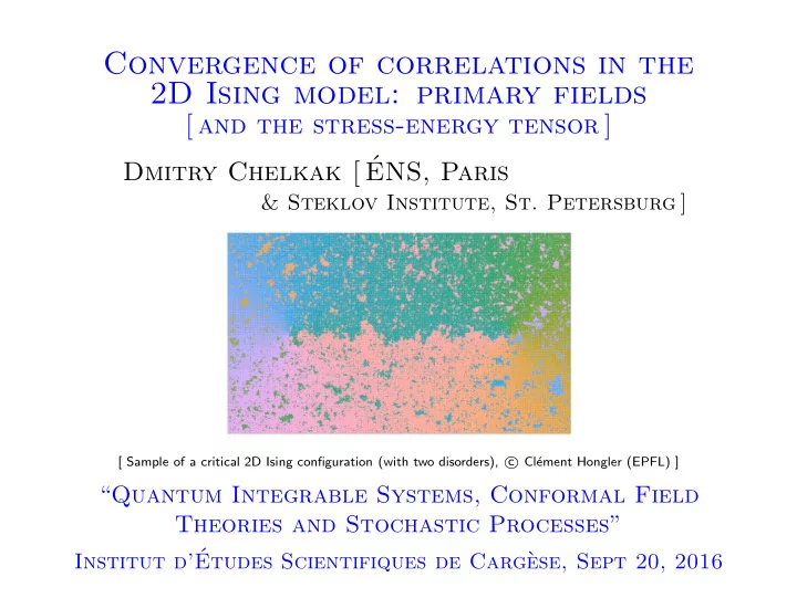
Convergence of correlations in the 2D Ising model: primary fields [ and the stress-energy tensor ] Dmitry Chelkak [ ´ ENS, Paris & Steklov Institute, St. Petersburg ] [ Sample of a critical 2D Ising configuration (with two disorders), c � Cl´ ement Hongler (EPFL) ] “Quantum Integrable Systems, Conformal Field Theories and Stochastic Processes” Institut d’´ Etudes Scientifiques de Carg` ese, Sept 20, 2016

2D Ising model: • N.n. 2D Ising model: combinatorics convergence ◦ dimers and fermionic observables of correlations ◦ discrete holomorphicity at criticality at criticality ◦ spinor observables and spin correlations ◦ spin-disorder formalism [ see also arXiv:1605.09035 ] • Spin correlations at criticality ◦ Riemann boundary value problems for holomorphic spinors in continuum ◦ Convergence [Ch.–Hongler–Izyurov] • Other primary fields: σ, µ, ε, ψ, ψ ◦ Convergence and fusion rules ◦ Construction of mixed correlations via Riemann boundary value problems • [ Stress-energy tensor ] ◦ (Some) discrete version of T and T ◦ Convergence [Ch.–Glazman–Smirnov] � Cl´ c ement Hongler (EPFL)

Nearest-neighbor Ising (or Lenz-Ising) model in 2D Definition: Lenz-Ising model on a planar graph G ∗ (dual to G ) is a random assignment of + / − spins to vertices of G ∗ (faces of G ) Q: I heard this is called a (site) percolation? A: .. according to the following probabilities: � � conf . σ ∈ {± 1 } V ( G ∗ ) � � β � P ∝ exp e = � uv � J uv σ u σ v ∝ � e = � uv � : σ u � = σ v x uv , where J uv > 0 are interaction constants assigned to edges � uv � , β = 1 / kT is the inverse temperature, and x uv = exp[ − 2 β J uv ].

Nearest-neighbor Ising (or Lenz-Ising) model in 2D Definition: Lenz-Ising model on a planar graph G ∗ (dual to G ) is a random assignment of + / − spins to vertices of G ∗ (faces of G ) Disclaimer: 2D, nearest-neighbor, no external magnetic field. � � conf . σ ∈ {± 1 } V ( G ∗ ) � � β � P ∝ exp e = � uv � J uv σ u σ v ∝ � e = � uv � : σ u � = σ v x uv , where J uv > 0 are interaction constants assigned to edges � uv � , β = 1 / kT is the inverse temperature, and x uv = exp[ − 2 β J uv ]. • It is also convenient to use the parametrization x uv = tan( 1 2 θ uv ). • Working with subgraphs of regular lattices , one can consider the homogeneous model in which all x uv are equal to each other.

Phase transition (e.g., on Z 2 ) E.g., Dobrushin boundary conditions: +1 on ( ab ) and − 1 on ( ba ): x < x crit x = x crit x > x crit • Ising (1925): no phase transition in 1D � doubts about 2+D; • Peierls (1936): existence of the phase transition in 2D; √ 2 − 1 = tan( 1 2 · π • Kramers-Wannier (1941): x self-dual = 4 ); √ • Onsager (1944): sharp phase transition at x crit = 2 − 1.

At criticality (e.g., on Z 2 ): ◦ Kaufman-Onsager(1948-49), Yang(1952): scaling exponent 1 8 for the magnetization. [via spin-spin correlations in Z 2 at x ↑ x crit ] ◦ At criticality, for Ω δ → Ω and u δ → u ∈ Ω, 1 8 as δ → 0. it should be E Ω δ [ σ u δ ] ≍ δ • Question: Convergence of (rescaled) spin correlations and conformal covariance of their scaling limits in arbitrary planar domains: x = x crit δ − n 8 · E Ω δ [ σ u 1 ,δ . . . σ u n ,δ ] → � σ u 1 . . . σ u n � Ω 1 � σ ϕ ( u 1 ) . . . σ ϕ ( u n ) � ϕ (Ω) · � n s =1 | ϕ ′ ( u s ) | = 8 • In the infinite-volume setup other techniques are available, notably “exact bosonization” approach due to J. Dub´ edat.

2D Ising model as a dimer model (on a non-bipartite graph) [Fisher, Kasteleyn (’60s+),..., Kenyon, Dub´ edat (’00s+),...] • Partition function Z = � � e = � uv � : σ u � = σ v x uv σ ∈{± 1 } V ( G ∗ ) • There exist various representa- tions of the 2D Ising model via dimers on an auxiliary graph

2D Ising model as a dimer model (on a non-bipartite graph) [Fisher, Kasteleyn (’60s+),..., Kenyon, Dub´ edat (’00s+),...] • Partition function Z = � � e = � uv � : σ u � = σ v x uv σ ∈{± 1 } V ( G ∗ ) • There exist various representa- tions of the 2D Ising model via dimers on an auxiliary graph G F

2D Ising model as a dimer model (on a non-bipartite graph) [Fisher, Kasteleyn (’60s+),..., Kenyon, Dub´ edat (’00s+),...] • Partition function Z = � � e = � uv � : σ u � = σ v x uv σ ∈{± 1 } V ( G ∗ ) • There exist various representa- tions of the 2D Ising model via dimers on an auxiliary graph: e.g. 1-to-2 | V ( G ) | correspondence of {± 1 } V ( G ∗ ) with dimers on this G F

2D Ising model as a dimer model (on a non-bipartite graph) [Fisher, Kasteleyn (’60s+),..., Kenyon, Dub´ edat (’00s+),...] • Partition function Z = � � e = � uv � : σ u � = σ v x uv σ ∈{± 1 } V ( G ∗ ) • There exist various representa- tions of the 2D Ising model via dimers on an auxiliary graph: e.g. 1-to-2 | V ( G ) | correspondence of {± 1 } V ( G ∗ ) with dimers on this G F • Kasteleyn’s theory: Z =Pf[ K ] [ K= − K ⊤ is a weighted adjacency matrix of F ] G

2D Ising model as a dimer model (on a non-bipartite graph) [Fisher, Kasteleyn (’60s+),..., Kenyon, Dub´ edat (’00s+),...] • Partition function Z = � � e = � uv � : σ u � = σ v x uv σ ∈{± 1 } V ( G ∗ ) • There exist various representa- tions of the 2D Ising model via dimers on an auxiliary graph: e.g. 1-to-2 | V ( G ) | correspondence of {± 1 } V ( G ∗ ) with dimers on this G F • Kasteleyn’s theory: Z =Pf[ K ] [ K= − K ⊤ is a weighted adjacency matrix of F ] G • Kac–Ward formula (1952–..., 1999–...): Z 2 = det[Id − T] , � exp[ i e ′ ) ] · ( x e x e ′ ) 1 / 2 2 wind( e , T e , e ′ = 0 [ is equivalent to the Kasteleyn theorem for dimers on F ] G

2D Ising model as a dimer model (on a non-bipartite graph) [Fisher, Kasteleyn (’60s+),..., Kenyon, Dub´ edat (’00s+),...] • Partition function Z = � � e = � uv � : σ u � = σ v x uv σ ∈{± 1 } V ( G ∗ ) • There exist various representa- tions of the 2D Ising model via dimers on an auxiliary graph: e.g. 1-to-2 | V ( G ) | correspondence of {± 1 } V ( G ∗ ) with dimers on this G F • Kasteleyn’s theory: Z =Pf[ K ] [ K= − K ⊤ is a weighted adjacency matrix of F ] G F ) ∼ • Note that V ( G = { G } o riented edges and o rners of • Local relations for the entries K − 1 a , e and K − 1 a , of the inverse Kasteleyn (or the inverse Kac–Ward) matrix: K · K − 1 = Id (an equivalent form of) the identity

Fermionic observables: combinatorial definition [Smirnov’00s] For an oriented edge a and a midedge z e (similarly, for a corner c ), � � e − i � 2 wind ( a � z e ) � F G ( a , z e ) := η a � uv �∈ ω x uv ω ∈ Conf G ( a , z e ) where η a denotes the (once and forever fixed) square root of the direction of a . 2 wind ( a � z e ) does not de- • The factor e − i pend on the way how ω is split into non- intersecting loops and a path a � z e . F : F G ( a , c ) = η c K − 1 • Via dimers on c , a G F G ( a , z e ) = η e K − 1 e , a + η e K − 1 e , a

Fermionic observables: combinatorial definition [Smirnov’00s] For an oriented edge a and a midedge z e (similarly, for a corner c ), � � e − i � 2 wind ( a � z e ) � F G ( a , z e ) := η a � uv �∈ ω x uv ω ∈ Conf G ( a , z e ) where η a denotes the (once and forever fixed) square root of the direction of a . • Local relations: at criticality, can be thought of as some (strong) form of discrete Cauchy–Riemann equations. • Boundary conditions F ( a , e ) ∈ η ¯ e R z ( e is oriented outwards) uniquely deter- mine F as a solution to an appropriate discrete Riemann-type boundary value problem.

Fermionic observables: combinatorial definition [Smirnov’00s] For an oriented edge a and a midedge z e (similarly, for a corner c ), � � e − i � 2 wind ( a � z e ) � F G ( a , z e ) := η a � uv �∈ ω x uv ω ∈ Conf G ( a , z e ) Fermionic observables per se can be used • to construct (discrete) martingales for growing interfaces and then to study their convergence to SLE curves [Smirnov(2006), ..., Ch.–Duminil-Copin –Hongler–Kemppainen–Smirnov(2013)] • to analyze the energy density field [Hongler–Smirnov, Hongler (2010)] e := δ − 1 · [ σ e + − ε ∞ e ] ε e − σ where e ± are the two neighboring faces separated by an edge e • but more involved ones are needed to study spin correlations

Energy density: convergence and conformal covariance • Three local primary fields: 1 , σ (spin), ε (energy density); Scaling exponents: 0 , 1 8 , 1 . • Theorem: [Hongler–Smirnov, Hongler (2010)] If Ω δ → Ω and e k ,δ → z k as δ → 0, then n � + δ − n · E + δ → 0 C n Ω δ [ ε e 1 ,δ . . . ε e n ,δ ] → ε · � ε z 1 . . . ε Ω z where C ε is a lattice-dependent constant, � ε z 1 . . . ε z n � + Ω = � ε ϕ ( z 1 ) . . . ε ϕ ( z n ) � + Ω ′ · � n s =1 | ϕ ′ ( u s ) | for any conformal mapping ϕ : Ω → Ω ′ , and H = i n · Pf ( z s − z m ) − 1 � 2 n n � + � � ε z 1 . . . ε s , m =1 , z s = z 2 n +1 − s . z • Ingredients: convergence of basic fermionic observables (via Riemann-type b.v.p.) and (built-in) Pfaffian formalism