
Statistically-Significant Correlations 11 Oct, 2014 2014-Schield-NNN4-slides.pdf 1
2014 NNN4 Statistically-Significant Correlations0F
1
Milo Schield Augsburg College Editor of www.StatLit.org
US Rep: International Statistical Literacy Project
Fall 2014 National Numeracy Network Conference
www.StatLit.org/pdf/2014-Schield-NNN4-Slides.pdf
Statistically-Significant Correlations
2014 NNN4 Statistically-Significant Correlations0F
2
Exact Solutions
For N random pairs from an uncorrelated bivariate normally-distributed distribution, the sampling distribution is not simple. Here are three common analytic approaches: 1.Fisher transformation (using LN and Arctanh), 2.an exact solution (using a Gamma function), or 3.Student-t distribution: t=rSqrt[(n-2)/(1-r^2)]; df=n-2
- For large n, the critical value of t (95% confidence) is 1.96.
- For small n, the critical value of t increases as n decreases.
None of these are simple or memorable.
2014 NNN4 Statistically-Significant Correlations0F
3
Sufficient Condition
Approach: Find an equation generating a minimum correlation for statistical-significance given N.
- 1. Given N, find the smallest value of r where the left
end of a 95% confidence interval is non-negative. Use calculator at www.vassarstats.net/rho.html or www.danielsoper.com/statcalc3/calc.aspx?id=44 For Daniels, use the results for a two-tailed test.
- 2. Generate correlation coefficient with simple model
- 3. Calculate error difference between calculated and
exact using the exact as the standard. If all errors are positive, then the model is sufficient.
2014 NNN4 Statistically-Significant Correlations0F
4
All errors positive means the model is sufficient.
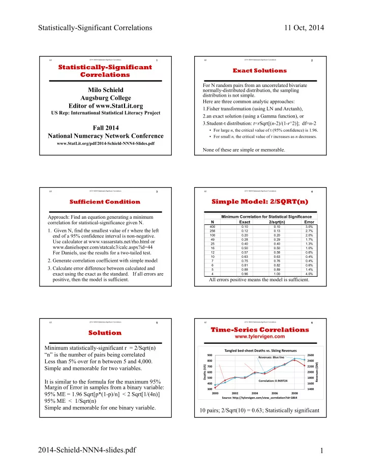
Simple Model: 2/SQRT(n)
Minimum Correlation for Statistical Significance N Exact 2/sqrt(n) Error
400 0.10 0.10 3.0% 256 0.12 0.13 2.7% 100 0.20 0.20 2.0% 49 0.28 0.29 1.7% 25 0.40 0.40 1.3% 16 0.50 0.50 1.0% 12 0.57 0.58 0.6% 10 0.63 0.63 0.4% 7 0.75 0.76 0.4% 6 0.81 0.82 0.6% 5 0.88 0.89 1.4% 4 0.96 1.00 4.0%
2014 NNN4 Statistically-Significant Correlations0F
5
Minimum statistically-significant r = 2/Sqrt(n) “n” is the number of pairs being correlated Less than 5% over for n between 5 and 4,000. Simple and memorable for two variables. It is similar to the formula for the maximum 95% Margin of Error in samples from a binary variable: 95% ME = 1.96 Sqrt[p*(1-p)/n] < 2 Sqrt[1/(4n)] 95% ME < 1/Sqrt(n) Simple and memorable for one binary variable.
Solution
2014 NNN4 Statistically-Significant Correlations0F
6
10 pairs; 2/Sqrt(10) = 0.63; Statistically significant
Time-Series Correlations
www.tylervigen.com
1400 1600 1800 2000 2200 2400 2600 300 400 500 600 700 800 900 2000 2002 2004 2006 2008 Revenues ($M) Deaths (US)
Tangled bed‐sheet Deaths vs. Skiing Revenues
Source: http://tylervigen.com/view_correlation?id=1864 Revenues: Blue line Correlation: 0.969724