
SLIDE 1
Methods and Algorithms for Advanced Process Control
STADIUS - Center for Dynamical Systems,
Signal Processing and Data Analytics Oscar Mauricio Agudelo
Controllability
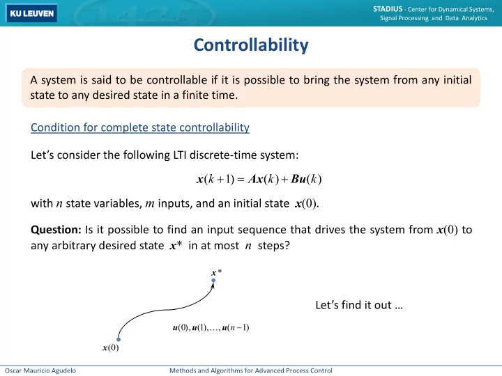
A system is said to be controllable if it is possible to bring the system from any initial state to any desired state in a finite time. Question: Is it possible to find an input sequence that drives the system from x(0) to any arbitrary desired state x* in at most n steps?
(0) x * x (0), (1), , ( 1) n − u u u