[PDF] - Contents Cournot and Bertrand Equilibria Single Market Assumption: PDF Document

SLIDE 1

1

S ystems

Analysis Laboratory

Helsinki University of Technology Oligopoly - Heikkilä T. / Murto P. - 1 Seminar on Microeconomics - Fall 1998

Single Market Assumption: Oligopoly

Tero Heikkilä, Pauli Murto 25.11.1998

S ystems

Analysis Laboratory

Helsinki University of Technology Oligopoly - Heikkilä T. / Murto P. - 2 Seminar on Microeconomics - Fall 1998

Background of Oligopoly

Oligopoly is a study of market interactions

with a small number of firms.

– “What is our Product’s Price and Output?”

grounded almost entirely on the theories of

Game Theory

Player 1

Our Firm

Player 2

Other Firms

The Market

S ystems

Analysis Laboratory

Helsinki University of Technology Oligopoly - Heikkilä T. / Murto P. - 4 Seminar on Microeconomics - Fall 1998

The strategic variable of the firms is output
Homogenous products with output levels y1

and y2, aggregate output Y= y1+y2

Firm i:
Interior Optimum, Nash-Cournot:

– f.o.c. – s.o.c.

Cournot Equilibrium

y i i i i

i

y y p y y y c y

max

( , ) ( ) ( ) π

1 2 1 2

= + −

∂π ∂

i i i i i

y y y p y y p y y y c y ( , ) ( ) '( ) '( )

1 2 1 2 1 2

= + + + − = ∂ π ∂

2 1 2 2 1 2 1 2

2

i i i i i

y y y p y y p y y y c y ( , ) '( ) ''( ) ''( ) = + + + − ≤

S ystems

Analysis Laboratory

Helsinki University of Technology Oligopoly - Heikkilä T. / Murto P. - 5 Seminar on Microeconomics - Fall 1998

Reaction Curve

∂π ∂

1 1 2 2 1

( ( ), ) f y y y ≡

f y y y y ' ( ) / /

1 2 2 1 1 2 2 1 1 2

= − ∂ π ∂ ∂ ∂ π ∂

F.o.c. for firm 1 determines it’s optimal

choice of output as a function y1= f1(y2).

Assuming sufficient regularity:
and differenitating the identity:
sign problem:

∂ π ∂ ∂

2 1 1 2 1

/ '( ) ''( ) y y p Y p Y y = +

S ystems

Analysis Laboratory

Helsinki University of Technology Oligopoly - Heikkilä T. / Murto P. - 6 Seminar on Microeconomics - Fall 1998

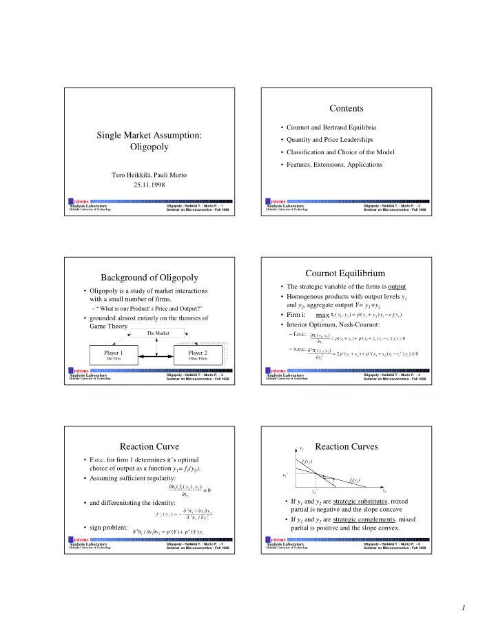
Reaction Curves

If y1 and y2 are strategic substitutes, mixed

partial is negative and the slope concave

If y1 and y2 are strategic complements, mixed

partial is positive and the slope convex.

y2 y1 f1(y2) f2(y1) y1

*

y2

*

SLIDE 2

2

S ystems

Analysis Laboratory

Helsinki University of Technology Oligopoly - Heikkilä T. / Murto P. - 7 Seminar on Microeconomics - Fall 1998

The Problem of

Stability

At time t=0,

firm 1 thinks:

After that, t=1, firm 2 thinks:
In general:
If it converges to the Cournot-Nash

Equilibrium, the illutrated equilibrium is stable.

Leads to dynamical system:

( , ) y y

1 2

y f y

1 1 1 2

= ( )

y f y

2 2 2 1 1

= ( ) y f y

i t i j t

=

−

( )

1

dy dt y y y

1 1 1 1 2 1

=       α ∂π ∂ ( , ) dy dt y y y

2 2 2 1 2 2

=       α ∂π ∂ ( , )

S ystems

Analysis Laboratory

Helsinki University of Technology Oligopoly - Heikkilä T. / Murto P. - 8 Seminar on Microeconomics - Fall 1998

The Solution of

Stability

Sufficient condition for local stability:
“Almost” necessary condition, method is

more like ad hoc.

Real dynamic analysis requires repeated

game analysis.

∂ π ∂ ∂ π ∂ ∂ ∂ π ∂ ∂ ∂ π ∂

2 1 1 2 2 1 1 2 2 2 1 2 2 2 2 2

y y y y y y > S ystems

Analysis Laboratory

Helsinki University of Technology Oligopoly - Heikkilä T. / Murto P. - 9 Seminar on Microeconomics - Fall 1998

Introduction of

Comparative Statics

Profit function of the firm 1 is shifted by a

parameter a.

and after differentiating

∂π ∂

1 1 2 1

( ( ), ( ), ) y a y a a y = ∂π ∂

2 1 2 2

( ( ), ( ), ) y a y a a y = ∂ π ∂ ∂ π ∂ ∂ ∂ π ∂ ∂ ∂ π ∂ ∂ ∂ ∂ ∂ ∂ π ∂ ∂

2 1 1 2 2 1 1 2 2 2 1 2 2 2 2 2 1 2 2 1 1

y y y y y y y a y a y a                       = −        

S ystems

Analysis Laboratory

Helsinki University of Technology Oligopoly - Heikkilä T. / Murto P. - 10 Seminar on Microeconomics - Fall 1998

Solution of

Comparative Statics

Cramer’s Rule gives:
The Sign :
Applied to duopoly model:

– marginal cost increase will reduce Cournot Equilibrium Output:

∂ ∂ ∂ π ∂ ∂ ∂ π ∂ ∂ ∂ π ∂ ∂ π ∂ ∂ π ∂ ∂ ∂ π ∂ ∂ ∂ π ∂ y a y a y y y y y y y y y

1 2 1 1 2 1 1 2 2 2 2 2 2 1 1 2 2 1 1 2 2 2 1 2 2 2 2 2

= −

sign y a sign y a ∂ ∂ ∂ π ∂ ∂

1 2 1 1

= ∂ π ∂ ∂

2 1 1

1 y a = − π1

1 2 1 2 1 1

( , , ) ( ) y y a p y y y ay = + −

S ystems

Analysis Laboratory

Helsinki University of Technology Oligopoly - Heikkilä T. / Murto P. - 11 Seminar on Microeconomics - Fall 1998

Monopoly vs. Pure Competition

Cournot f.o.c. for several firms:

p Y p Y y c y

i i i

( ) '( ) '( ) + − = 0 Y yi

i n

=

∑

1

p Y dp dY y p c y

i i i

( ) '( ) 1+       = p Y dp dY Y p s c y

i i i

( ) '( ) 1+       = s y Y

i i

= p Y dp dY s c y

i i i

( ) '( ) 1+       = ε ε = p Y

Application of Cournot:

S ystems

Analysis Laboratory

Helsinki University of Technology Oligopoly - Heikkilä T. / Murto P. - 12 Seminar on Microeconomics - Fall 1998

Welfare

Cournot industry produces inefficiently low

level of output since price exceeds marginal cost.

The ouput level of symmetric Cournot

equilibrium with constant marginal costs maximizes:

A competitive industry maximizes utility

minus costs, monopoly maximizes profits.

[ ]

W Y p Y c Y n U Y cY ( ) ( ) ( ) ( ) = − + + − 1

SLIDE 3

3

S ystems

Analysis Laboratory

Helsinki University of Technology Oligopoly - Heikkilä T. / Murto P. - 13 Seminar on Microeconomics - Fall 1998

Bertrand Equilibrium

The relevant strategic Variable: Price
Constant marginal costs, assume c2 > c1 ,
Demand curve facing Firm 1:

d p p D p D p

1 1 2 1 1

2 ( , ) ( ), ( ) / , , =      if if if

p p

1 2

< p p

1 2

= p p

1 2

> c2 c1

$

p2 p1

{

π 2

?

S ystems

Analysis Laboratory

Helsinki University of Technology Oligopoly - Heikkilä T. / Murto P. - 14 Seminar on Microeconomics - Fall 1998

Characteristics of Bertrand

One-shot game: sealed bids, one or some get

all and the game ends.

For the Firm 1 p1=c2 as long as p1>c1.
Mixed strategies:

– propability distribution over the prices of the

ther companys

– choose own probability distribution to maximise expected profits S ystems

Analysis Laboratory

Helsinki University of Technology Oligopoly - Heikkilä T. / Murto P. - 15 Seminar on Microeconomics - Fall 1998

Example: A Model of Sales

The Mixed Strategy Equilibrium

Each firm has zero marginal costs and fixed costs k.
On the market exists:

– Informed Customers ( I ) – Uninformed Costomers ( U )

Symmetric Equilibrium. Each Firm has the same

mixed Strategy.

F(p) cumulative distribution function of the price in

Equilibrium strategy, f(p) propability density function. S ystems

Analysis Laboratory

Helsinki University of Technology Oligopoly - Heikkilä T. / Murto P. - 16 Seminar on Microeconomics - Fall 1998

Example: A Model of Sales

Stating Profit Equation

Expected Profits:
Every Price, actually charged in the

equilibrium strategy, must yield the same expected profit:

or

π = − + + − p F p I U pF p U k ( ( ))( ) ( ) 1 [ ]

π = − + + −

∞

∫

p F p I U pF p U k f p dp ( ( ))( ) ( ) ( ) 1

F p p I U k pI ( ) ( ) = + − − π

S ystems

Analysis Laboratory

Helsinki University of Technology Oligopoly - Heikkilä T. / Murto P. - 17 Seminar on Microeconomics - Fall 1998

Example: A Model of Sales

The End of the Solving

The propability that a firm would charge a

price less or equal to r is 1:

– which gives: – and after substituting:

Setting

, we get

Expression is zero at
so

F p p I U rU pI ( ) ( ) = + −

u U I = /

F p ( ) = 0 F p ( ) = 1 p p ≤ p r ≥

p ru u = + / ( ) 1

F p u ru p ( ) = + − 1

π = − rU k F r ( ) = 1 S ystems

Analysis Laboratory

Helsinki University of Technology Oligopoly - Heikkilä T. / Murto P. - 18 Seminar on Microeconomics - Fall 1998

The Grade of Substitutes ,

Introduction of Variables

Consumer’s inverse demand functions:
Direct demand functions:
Index of product differentiation:

p y y

1 1 1 1 2

= − − α β γ p y y

2 2 1 2 2

= − − α γ β y a b p cp

1 1 1 1 2

= − + y a cp b p

2 2 1 2 2

= + −

γ β β

2 1 2

SLIDE 4

4

S ystems

Analysis Laboratory

Helsinki University of Technology Oligopoly - Heikkilä T. / Murto P. - 19 Seminar on Microeconomics - Fall 1998

The Grade of Substitutes

Cournot Competitor maximizes:
and gets
Bertrand Competitor maximizes:
and gets

( ) α β γ

1 1 1 2 1

− − y y y ( ) a b p cp p

1 1 1 2 1

− +

y y

1 1 2 1

2 = − α γ β p a cp b

1 1 2 1

2 = +

S ystems

Analysis Laboratory

Helsinki University of Technology Oligopoly - Heikkilä T. / Murto P. - 20 Seminar on Microeconomics - Fall 1998

Quantity Leadership

Also known as Stackelberg model
In the book, only 2 players are assumed
A two stage model, where one player, ‘the

leader’, can move before the other one

Leader can optimize his output given the fact

that the other one will react optimally

Leader can take the reaction of the follower into

account when deciding his action

S ystems

Analysis Laboratory

Helsinki University of Technology Oligopoly - Heikkilä T. / Murto P. - 21 Seminar on Microeconomics - Fall 1998

Quantity Leadership

(cont.)

The follower maximizes:
The leader maximizes:

π2

2 1 2 2 2 2

( ) ( ) ( ) y p y y y c y = + −

y g y

2 1

= ( )

π1

1 1 1 1 1 1

( ) ( ( )) ( ) y p y g y y c y = + −

S ystems

Analysis Laboratory

Helsinki University of Technology Oligopoly - Heikkilä T. / Murto P. - 22 Seminar on Microeconomics - Fall 1998

Firms prefer to be Leaders

Assume heterogenous goods
If following assumptions satisfied,

– A1: Substitute products – A2: Downward sloping reaction curves

then a firm always weakly prefers to be a leader rather than a follower

These assumptions include as a special case

homogeneous goods

S ystems

Analysis Laboratory

Helsinki University of Technology Oligopoly - Heikkilä T. / Murto P. - 23 Seminar on Microeconomics - Fall 1998

One Leader - many Followers

One player acts first, others follow

simultaneously

The leader sets the quantity knowing that the

followers take this as given

Followers play Nash among themselves

S ystems

Analysis Laboratory

Helsinki University of Technology Oligopoly - Heikkilä T. / Murto P. - 24 Seminar on Microeconomics - Fall 1998

One Leader - three Followers

(all have similar cost functions) Profit of the leader and price as a function of

utput of the leader

10 20 30 40 50 60 70 80 90 100

10 20 30 40 50 60 70 profit price market demand

SLIDE 5

5

S ystems

Analysis Laboratory

Helsinki University of Technology Oligopoly - Heikkilä T. / Murto P. - 25 Seminar on Microeconomics - Fall 1998

One Leader, three Followers

(all have similar cost functions) Outputs of the followers as functions of

utput of the leader

5 10 15 20 25 30 2 4 6 8 10 12 14 16 18 20 22 24 26 28 30 32 34 36 38 X qi q3 q2 q1

S ystems

Analysis Laboratory

Helsinki University of Technology Oligopoly - Heikkilä T. / Murto P. - 26 Seminar on Microeconomics - Fall 1998

Stackelberg vs. Cournot Equilibria

(4 players with similar costs)

S-C (Leader/Follower) Cournot Output

16.5 / 4.51 6.83

Profit

96.90 / 26.50 65.13

Total Quantity

30.04 27.32

Price

30.87 34.54

S ystems

Analysis Laboratory

Helsinki University of Technology Oligopoly - Heikkilä T. / Murto P. - 27 Seminar on Microeconomics - Fall 1998

Price Leadership

One firm sets the price, the other firm then takes

this as given

Assume heterogeneous products:

= demand for output of firm i

x p p

i(

, )

1 2

S ystems

Analysis Laboratory

Helsinki University of Technology Oligopoly - Heikkilä T. / Murto P. - 28 Seminar on Microeconomics - Fall 1998

Price Leadership

(cont.)

Follower maximizes:
Leader maximizes:

π2

2 2 2 1 2 2 2 1 2

( ) ( , ) ( ( , )) p p x p p c x p p = −

p g p

2 1

= ( )

π1

1 1 1 1 1 1 1 1 1

( ) ( , ( )) ( ( , ( ))) p p x p g p c x p g p = −

S ystems

Analysis Laboratory

Helsinki University of Technology Oligopoly - Heikkilä T. / Murto P. - 29 Seminar on Microeconomics - Fall 1998

Special case: Identical Products

The follower must choose
The follower can, however, choose the output at

that price:

The leader’s output is then the residual demand:
So, the leader maximizes:

max

p p

2 1

=

S p

2 1

( ) r p x p S p ( ) ( ) ( )

1 1 1 2 1

= −

p r p c r p

1 1 1 1

( ) ( ( )) −

S ystems

Analysis Laboratory

Helsinki University of Technology Oligopoly - Heikkilä T. / Murto P. - 30 Seminar on Microeconomics - Fall 1998

Firms prefer to be Followers

If both firms have upward sloping reaction

functions, then if one prefers to be a leader, the

ther must prefer to be a follower
If both firms have identical cost and demand

functions and reaction curves are upward sloping, then each player prefers to be the follower to being the leader

SLIDE 6

6

S ystems

Analysis Laboratory

Helsinki University of Technology Oligopoly - Heikkilä T. / Murto P. - 31 Seminar on Microeconomics - Fall 1998

Classification

Strategic Space Price Quantity, Output Level of Information Others’ Choices Known Others’ Choices Unknown

Cournot Bertrand Quantity Leadership Price Leadership

S ystems

Analysis Laboratory

Helsinki University of Technology Oligopoly - Heikkilä T. / Murto P. - 32 Seminar on Microeconomics - Fall 1998

Choice of the Model

One-shot: Strategic Variable should be

somehow slow to change.

– “output” - capacity

Two-stage game: Cournot - Bertrand

– Cournot Equilibrium S ystems

Analysis Laboratory

Helsinki University of Technology Oligopoly - Heikkilä T. / Murto P. - 33 Seminar on Microeconomics - Fall 1998

Conjectural Variations

The optimal quantity choice of Stackelberg

Leader’s f.o.c.:

Conjectural variatiation:

[ ]

p Y p Y y c y ( ) '( ) '( ) + + = 1

12 1 1 1

ν

[ ]

p Y p Y f y y c y ( ) '( ) '( ) '( ) + + = 1

2 1 1 1 1

ν12

2 1

= f y '( )

ν12 =

Cournot Model

ν12 1 = − - The competetive model ν12 = slope of firm 2’s reaction curve

Stackelberg

model ν12

2 1

= y y /

The collusice

equilibium

S ystems

Analysis Laboratory

Helsinki University of Technology Oligopoly - Heikkilä T. / Murto P. - 34 Seminar on Microeconomics - Fall 1998

Collusion

Oligopoly producers can form a cartel to

maximize joint profits

The situation is strategically similar to Prisoner’s

Dilemma

To have a stable cooperative solution, there has

to be a credible punishment threat

The punishment can be that the firm will keep

its market share constant even if the other firm cheats

S ystems

Analysis Laboratory

Helsinki University of Technology Oligopoly - Heikkilä T. / Murto P. - 35 Seminar on Microeconomics - Fall 1998

Repeated Oligopoly Games

All considerations so far have been one-shot

games

The repeated oligopoly analysis follows the

analysis of repeated Prisoner’s Dilemma

– The cooperative outcome: cartel – The punishment: Cournot-solution S ystems

Analysis Laboratory

Helsinki University of Technology Oligopoly - Heikkilä T. / Murto P. - 36 Seminar on Microeconomics - Fall 1998

Repeated Oligopoly

(cont.)

In finitely repeated games, the Cournot equilibrium is the
nly subgame perfect equilibrium
In infinitely repeated games, the strategies ‘cooperate as

long as the other will, and otherwise go to Cournot level forever’ make a subgame perfect equilibrium if:

There are, however, other subgame perfect equilibria

strategies as well

δ π π π π > − −

∗ 2 2 2 2 d d c

SLIDE 7

7

S ystems

Analysis Laboratory

Helsinki University of Technology Oligopoly - Heikkilä T. / Murto P. - 37 Seminar on Microeconomics - Fall 1998

Threat of Entry

Assume there is a firm producing in the market,

and some other firm(s) who might enter the market

Pricing to prevent entry is called limit pricing
There is no sense if all the firms have perfect

information

However, if the potential entrants don’t know the

cost structure of the currently producing firm, pricing can be used to prevent entry in some cases (see the example in the book)

S ystems

Analysis Laboratory

Helsinki University of Technology Oligopoly - Heikkilä T. / Murto P. - 38 Seminar on Microeconomics - Fall 1998