contents foundations of artificial intelligence
play

Contents Foundations of Artificial Intelligence Introduction to - PowerPoint PPT Presentation

Contents Foundations of Artificial Intelligence Introduction to Utility Theory 1 12. Acting under Uncertainty Choosing Individual Actions 2 Maximizing Expected Utility Sequential Decision Problems 3 Wolfram Burgard, Bernhard Nebel, and


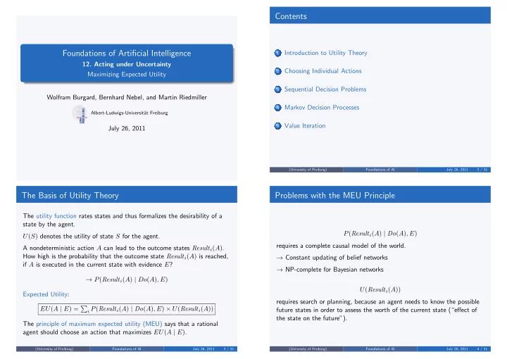
  1. Contents Foundations of Artificial Intelligence Introduction to Utility Theory 1 12. Acting under Uncertainty Choosing Individual Actions 2 Maximizing Expected Utility Sequential Decision Problems 3 Wolfram Burgard, Bernhard Nebel, and Martin Riedmiller Markov Decision Processes 4 Albert-Ludwigs-Universit¨ at Freiburg Value Iteration 5 July 26, 2011 (University of Freiburg) Foundations of AI July 26, 2011 2 / 31 The Basis of Utility Theory Problems with the MEU Principle The utility function rates states and thus formalizes the desirability of a state by the agent. P ( Result i ( A ) | Do ( A ) , E ) U ( S ) denotes the utility of state S for the agent. requires a complete causal model of the world. A nondeterministic action A can lead to the outcome states Result i ( A ) . How high is the probability that the outcome state Result i ( A ) is reached, → Constant updating of belief networks if A is executed in the current state with evidence E ? → NP-complete for Bayesian networks → P ( Result i ( A ) | Do ( A ) , E ) U ( Result i ( A )) Expected Utility: requires search or planning, because an agent needs to know the possible EU ( A | E ) = � i P ( Result i ( A ) | Do ( A ) , E ) × U ( Result i ( A )) future states in order to assess the worth of the current state (“effect of the state on the future”). The principle of maximum expected utility (MEU) says that a rational agent should choose an action that maximizes EU ( A | E ) . (University of Freiburg) Foundations of AI July 26, 2011 3 / 31 (University of Freiburg) Foundations of AI July 26, 2011 4 / 31
  2. The Axioms of Utility Theory (1) The Axioms of Utility Theory (2) Justification of the MEU principle, i.e., maximization of the average utility. Given states A , B , C Scenario = Lottery L Orderability Possible outcomes = possible prizes ( A ≻ B ) ∨ ( B ≻ A ) ∨ ( A ∼ B ) The outcome is determined by chance An agent should know what it wants: it must either prefer one of the 2 L = [ p 1 , C 1 ; p 2 , C 2 ; . . . ; p n , C n ] lotteries or be indifferent to both. Example: Transitivity Lottery L with two outcomes, C 1 and C 2 : ( A ≻ B ) ∧ ( B ≻ C ) ⇒ ( A ≻ C ) L = [ p, C 1 ; 1 − p, C 2 ] Violating transitivity causes irrational behavior: A ≻ B ≻ C ≻ A . The agent has A and would pay to exchange it for C . C would do the same Preference between lotteries: for A . L 1 ≻ L 2 The agent prefers L 1 over L 2 → The agent loses money this way. L 1 ∼ L 2 The agent is indifferent between L 1 and L 2 L 1 � L 2 The agent prefers L 1 or is indifferent between L 1 and L 2 (University of Freiburg) Foundations of AI July 26, 2011 5 / 31 (University of Freiburg) Foundations of AI July 26, 2011 6 / 31 The Axioms of Utility Theory (3) The Axioms of Utility Theory (4) Continuity Monotonicity A ≻ B ≻ C ⇒ ∃ p [ p, A ; 1 − p, C ] ∼ B A ≻ B ⇒ ( p ≥ q ⇔ [ p, A ; 1 − p, B ] � [ q, A ; 1 − q, B ]) If some state B is between A and C in preference, then there is some If an agent prefers the outcome A , then it must also prefer the lottery probability p for which the agent is indifferent between getting B for that has a higher probability for A . sure and the lottery that yields A with probability p and C with probability 1 − p . Decomposability [ p, A ; 1 − p, [ q, B ; 1 − q, C ]] ∼ [ p, A ; (1 − p ) q, B ; (1 − p (1 − q ) , C ] Substitutability An agent should not automatically prefer lotteries with more choice A ∼ B ⇒ [ p, A ; 1 − p, C ] ∼ [ p, B ; 1 − p, C ] points (“no fun in gambling”). Simpler lotteries can be replaced by more complicated ones, without changing the indifference factor. (University of Freiburg) Foundations of AI July 26, 2011 7 / 31 (University of Freiburg) Foundations of AI July 26, 2011 8 / 31

  3. Utility Functions and Axioms Possible Utility Functions From economic models: The axioms only make statements about preferences. U U The existence of a utility function follows from the axioms! Utility Principle If an agent’s preferences obey the axioms, then there exists a function U : S �→ R with o o o o o o o o U ( A ) > U ( B ) ⇔ A ≻ B o $ $ o o U ( A ) = U ( B ) ⇔ A ∼ B o �150,000 800,000 o o Maximum Expected Utility Principle U ([ p 1 , S 1 ; . . . ; p n , S n ]) = � i p i U ( S i ) o (a) (b) How do we design utility functions that cause the agent to act as desired? (University of Freiburg) Foundations of AI July 26, 2011 9 / 31 (University of Freiburg) Foundations of AI July 26, 2011 10 / 31 Assessing Utilities Sequential Decision Problems (1) 3 + 1 Scaling and normalizing: Best possible price U ( S ) = u max = 1 2 − 1 Worst catastrophe U ( S ) = u min = 0 START 1 We obtain intermediate utilities of intermediate outcomes by asking the 1 2 3 4 agent about its preference between a state S and a standard lottery [ p, u max ; 1 − p, u min ] . Beginning in the start state the agent must choose an action at each The probability p is adjusted until the agent is indifferent between S and time step. the standard lottery. The interaction with the environment terminates if the agent reaches Assuming normalized utilities, the utility of S is given by p . one of the goal states (4,3) (reward of +1) or (4,2) (reward -1). Each other location has a reward of -.04. In each location the available actions are Up , Down , Left , Right . (University of Freiburg) Foundations of AI July 26, 2011 11 / 31 (University of Freiburg) Foundations of AI July 26, 2011 12 / 31

  4. Sequential Decision Problems (2) Markov Decision Problem (MDP) Given a set of states in an accessible, stochastic environment, an MDP is Deterministic version: All actions always lead to the next square in the defined by selected direction, except that moving into a wall results in no change in position. Initial state S 0 Transition Model T ( s, a, s ′ ) Stochastic version: Each action achieves the intended effect with Reward function R ( s ) probability 0.8, but the rest of the time, the agent moves at right angles to the intended direction. Transition model: T ( s, a, s ′ ) is the probability that state s ′ is reached, if action a is executed in state s . 0.8 Policy: Complete mapping π that specifies for each state s which action 0.1 0.1 π ( s ) to take. Wanted : The optimal policy π ∗ is the policy that maximizes the expected utility. (University of Freiburg) Foundations of AI July 26, 2011 13 / 31 (University of Freiburg) Foundations of AI July 26, 2011 14 / 31 Optimal Policies (1) Optimal Policies (2) Given the optimal policy, the agent uses its current percept that tells it its current state. It then executes the action π ∗ ( s ) . We obtain a simple reflex agent that is computed from the information used for a utility-based agent. Optimal policy for our MDP: 3 +1 2 –1 1 1 2 3 4 How to compute optimal policies? (University of Freiburg) Foundations of AI July 26, 2011 15 / 31 (University of Freiburg) Foundations of AI July 26, 2011 16 / 31

  5. Finite and Infinite Horizon Problems Assigning Utilities to State Sequences Performance of the agent is measured by the sum of rewards for the states visited. For stationary systems there are just two ways to assign utilities to state sequences. To determine an optimal policy we will first calculate the utility of each state and then use the state utilities to select the optimal action for Additive rewards: each state. U h ([ s 0 , s 1 , s 2 , . . . ]) = R ( s 0 ) + R ( s 1 ) + R ( s 2 ) + · · · The result depends on whether we have a finite or infinite horizon problem. Discounted rewards: U h ([ s 0 , s 1 , s 2 , . . . ]) = R ( s 0 ) + γR ( s 1 ) + γ 2 R ( s 2 ) + · · · Utility function for state sequences: U h ([ s 0 , s 1 , . . . , s n ]) Finite horizon: U h ([ s 0 , s 1 , . . . , s N + k ]) = U h ([ s 0 , s 1 , . . . , s N ]) for all The term γ ∈ [0 , 1[ is called the discount factor. k > 0 . With discounted rewards the utility of an infinite state sequence is For finite horizon problems the optimal policy depends on the horizon N always finite. The discount factor expresses that future rewards have and therefore is called nonstationary. less value than current rewards. In infinite horizon problems the optimal policy only depends on the current state and therefore is stationary. (University of Freiburg) Foundations of AI July 26, 2011 17 / 31 (University of Freiburg) Foundations of AI July 26, 2011 18 / 31 Utilities of States Example The utilities of the states in our 4 × 3 world with γ = 1 and R ( s ) = − 0 . 04 The utility of a state depends on the utility of the state sequences that for non-terminal states: follow it. Let U π ( s ) be the utility of a state under policy π . Let s t be the state of the agent after executing π for t steps. Thus, the 3 0.812 0.868 0.918 + 1 utility of s under π is � ∞ � 2 0.762 0.660 –1 � U π ( s ) = E γ t R ( s t ) | π, s 0 = s t =0 1 0.705 0.655 0.611 0.388 The true utility U ( s ) of a state is U π ∗ ( s ) . R ( s ) is the short-term reward for being in s and 1 2 3 4 U ( s ) is the long-term total reward from s onwards. (University of Freiburg) Foundations of AI July 26, 2011 19 / 31 (University of Freiburg) Foundations of AI July 26, 2011 20 / 31

Download Presentation
Download Policy: The content available on the website is offered to you 'AS IS' for your personal information and use only. It cannot be commercialized, licensed, or distributed on other websites without prior consent from the author. To download a presentation, simply click this link. If you encounter any difficulties during the download process, it's possible that the publisher has removed the file from their server.

Recommend


More recommend