SLIDE 1
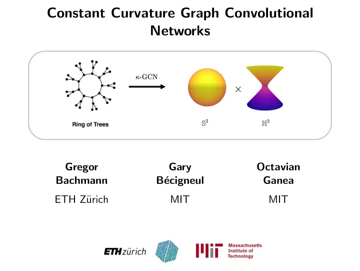
Constant Curvature Graph Convolutional Networks
Gregor Bachmann ETH Z¨ urich Gary B´ ecigneul MIT Octavian Ganea MIT
SLIDE 2
Overview
SLIDE 3 Overview
- Embeddings of graphs into hyperbolic and spherical space
and their products
SLIDE 4 Overview
- Embeddings of graphs into hyperbolic and spherical space
and their products
- Extend gyrovector framework to spherical geometry and
provide a unifying formalism
SLIDE 5 Overview
- Embeddings of graphs into hyperbolic and spherical space
and their products
- Extend gyrovector framework to spherical geometry and
provide a unifying formalism
- Introduce graph neural networks producing embeddings in
product spaces
SLIDE 6 Overview
- Embeddings of graphs into hyperbolic and spherical space
and their products
- Extend gyrovector framework to spherical geometry and
provide a unifying formalism
- Introduce graph neural networks producing embeddings in
product spaces
- Differentiable transitions in geometry during training in each
component
SLIDE 7
Graphs
SLIDE 8 Graphs
- Lots of data available in the form of graphs (social networks,
railway tracks, phylogenetic trees etc.)
SLIDE 9 Graphs
- Lots of data available in the form of graphs (social networks,
railway tracks, phylogenetic trees etc.)
SLIDE 10 Graphs
- Lots of data available in the form of graphs (social networks,
railway tracks, phylogenetic trees etc.)
- Node set V = {1, . . . , n} and adjacency matrix A ∈ Rn×n
SLIDE 11
Where to Embed Graphs?
SLIDE 12 Where to Embed Graphs?
- Euclidean geometry not suitable for many graphs
SLIDE 13 Where to Embed Graphs?
- Euclidean geometry not suitable for many graphs
SLIDE 14 Where to Embed Graphs?
- Euclidean geometry not suitable for many graphs
- Graph distance dG(i, j) = ”Shortest path from i to j” not
respected in Euclidean embedding
SLIDE 15 Where to Embed Graphs?
- Euclidean geometry not suitable for many graphs
- Graph distance dG(i, j) = ”Shortest path from i to j” not
respected in Euclidean embedding
- Arbitrary low distortion in spherical and hyperbolic space
SLIDE 16
Non-Euclidean Geometry
SLIDE 17 Non-Euclidean Geometry
- Focus on constant sectional curvature manifolds
SLIDE 18 Non-Euclidean Geometry
- Focus on constant sectional curvature manifolds
- Well-studied in the field of Differential Geometry
SLIDE 19 Non-Euclidean Geometry
- Focus on constant sectional curvature manifolds
- Well-studied in the field of Differential Geometry
- Computationally attractive expressions for distance,
exponential map etc.
SLIDE 20
Hyperbolic Space as Poincar´ e Ball
SLIDE 21 Hyperbolic Space as Poincar´ e Ball
1 √c } with curvature −c equipped with
Riemannian tensor gc
x = 4 (1−c||x||2)2 1
SLIDE 22 Hyperbolic Space as Poincar´ e Ball
1 √c } with curvature −c equipped with
Riemannian tensor gc
x = 4 (1−c||x||2)2 1
- Projection of hyperboloid
SLIDE 23 Hyperbolic Space as Poincar´ e Ball
1 √c } with curvature −c equipped with
Riemannian tensor gc
x = 4 (1−c||x||2)2 1
- Projection of hyperboloid
- dc
H (x, y) = 1 √c cosh−1
2 c ||x−y||2 2
( 1
c −||x||2 2)( 1 c −||y||2 2)
H
Projection of hyperboloid [4]
SLIDE 24
Gyrospace Structure
SLIDE 25 Gyrospace Structure
- Next best thing to a vector space
SLIDE 26 Gyrospace Structure
- Next best thing to a vector space
- Vector addition x + y → x ⊕c y
SLIDE 27 Gyrospace Structure
- Next best thing to a vector space
- Vector addition x + y → x ⊕c y
- Scalar multiplication rx → r ⊗c x
SLIDE 28 Gyrospace Structure
- Next best thing to a vector space
- Vector addition x + y → x ⊕c y
- Scalar multiplication rx → r ⊗c x
- Geodesic γx−
→y(t) = x ⊕c (t ⊗c (−x ⊕c y))
SLIDE 29
Spherical Space as Stereographic Projection
SLIDE 30 Spherical Space as Stereographic Projection
- Stereographic projection of Sd+1 ∼
= Rd + gc
x where
gc
x = 4 (1+c||x||2)2 1
SLIDE 31 Spherical Space as Stereographic Projection
- Stereographic projection of Sd+1 ∼
= Rd + gc
x where
gc
x = 4 (1+c||x||2)2 1
S (x, y) = 1 √c cos−1
2 c ||x−y||2 2
( 1
c +||x||2 2)( 1 c +||y||2 2)
SLIDE 32 Spherical Space as Stereographic Projection
- Stereographic projection of Sd+1 ∼
= Rd + gc
x where
gc
x = 4 (1+c||x||2)2 1
S (x, y) = 1 √c cos−1
2 c ||x−y||2 2
( 1
c +||x||2 2)( 1 c +||y||2 2)
SLIDE 33
Our Contributions: 1) Unified Formalism
SLIDE 34 Our Contributions: 1) Unified Formalism
- κ-stereographic model for any κ ∈ R:
std
κ = {x ∈ Rd | −κx2 2 < 1}
SLIDE 35 Our Contributions: 1) Unified Formalism
- κ-stereographic model for any κ ∈ R:
std
κ = {x ∈ Rd | −κx2 2 < 1}
Rd std
κ
x ⊕κ y x + y
(1−2κxT y−κ||y||2)x+(1+κ||x||2)y 1−2κxT y+κ2||x||2||y||2
r ⊗κ x rx tanκ (r · tan−1
κ ||x||) x ||x||
γx→y(t) x + t(y − x) x ⊕κ (t ⊗κ (−x ⊕κ y))
SLIDE 36 Our Contributions: 1) Unified Formalism
- κ-stereographic model for any κ ∈ R:
std
κ = {x ∈ Rd | −κx2 2 < 1}
Rd std
κ
x ⊕κ y x + y
(1−2κxT y−κ||y||2)x+(1+κ||x||2)y 1−2κxT y+κ2||x||2||y||2
r ⊗κ x rx tanκ (r · tan−1
κ ||x||) x ||x||
γx→y(t) x + t(y − x) x ⊕κ (t ⊗κ (−x ⊕κ y))
- More unifying expressions for distance, exponential map
- etc. in our paper!
SLIDE 37
Our Contributions: 2) Matrix Multiplications
SLIDE 38 Our Contributions: 2) Matrix Multiplications
- Embeddings X where Xi• ∈ std
κ, W ∈ Rd×k and A ∈ Rn×n
SLIDE 39 Our Contributions: 2) Matrix Multiplications
- Embeddings X where Xi• ∈ std
κ, W ∈ Rd×k and A ∈ Rn×n
- Right matrix multiplication XW acts on columns X•i
Thus lift to tangent space at zero: (X ⊗κ W )i• = expκ
0 ((logκ 0(X)W )i•)
SLIDE 40 Our Contributions: 2) Matrix Multiplications
- Embeddings X where Xi• ∈ std
κ, W ∈ Rd×k and A ∈ Rn×n
- Right matrix multiplication XW acts on columns X•i
Thus lift to tangent space at zero: (X ⊗κ W )i• = expκ
0 ((logκ 0(X)W )i•)
- Introduced in [2], we extended it to spherical spaces
SLIDE 41
Our Contributions: 2) Matrix Multiplications
SLIDE 42 Our Contributions: 2) Matrix Multiplications
- Left matrix multiplication AX acts on rows Xi•:
(AX)i• = Ai1X1• + · · · + AinXn•
SLIDE 43 Our Contributions: 2) Matrix Multiplications
- Left matrix multiplication AX acts on rows Xi•:
(AX)i• = Ai1X1• + · · · + AinXn•
- Idea: Reduce problem of linear combination to definition of
a non-euclidean midpoint
SLIDE 44 Our Contributions: 2) Matrix Multiplications
- Left matrix multiplication AX acts on rows Xi•:
(AX)i• = Ai1X1• + · · · + AinXn•
- Idea: Reduce problem of linear combination to definition of
a non-euclidean midpoint
SLIDE 45
Our Contributions: 2) Matrix Multiplications
SLIDE 46 Our Contributions: 2) Matrix Multiplications
- Leverage gyromidpoint for hyperbolic space and extend it to
std
κ:
mκ(x1, · · · , xn; α) = 1 2 ⊗κ n
αiλκ
xi
n
j=1 αj(λκ xj − 1)xi
SLIDE 47 Our Contributions: 2) Matrix Multiplications
- Leverage gyromidpoint for hyperbolic space and extend it to
std
κ:
mκ(x1, · · · , xn; α) = 1 2 ⊗κ n
αiλκ
xi
n
j=1 αj(λκ xj − 1)xi
- Define left matrix multiplication row-wise:
(A ⊠κ X)i• := (
Aij) ⊗κ mκ(X1•, · · · , Xn•; Ai•)
SLIDE 48 Our Contributions: 2) Matrix Multiplications
- Leverage gyromidpoint for hyperbolic space and extend it to
std
κ:
mκ(x1, · · · , xn; α) = 1 2 ⊗κ n
αiλκ
xi
n
j=1 αj(λκ xj − 1)xi
- Define left matrix multiplication row-wise:
(A ⊠κ X)i• := (
Aij) ⊗κ mκ(X1•, · · · , Xn•; Ai•)
- Same scaling behaviour: dκ(0, r ⊗κ x) = r · dκ(0, x)
SLIDE 49
Gyromidpoint for Varying Curvature
SLIDE 50
Our Contributions: 3) Differentiable Interpolation
SLIDE 51 Our Contributions: 3) Differentiable Interpolation
- All quantities recover their Euclidean counterpart for κ −
→ 0±
SLIDE 52 Our Contributions: 3) Differentiable Interpolation
- All quantities recover their Euclidean counterpart for κ −
→ 0±
- We proved an even stronger result:
SLIDE 53 Our Contributions: 3) Differentiable Interpolation
- All quantities recover their Euclidean counterpart for κ −
→ 0±
- We proved an even stronger result:
Differentiability of std
κ w.r.t. κ around 0
The first order derivatives at 0− and 0+ w.r.t. to κ of all the mentioned quantities exist and are equal.
SLIDE 54 Our Contributions: 3) Differentiable Interpolation
- All quantities recover their Euclidean counterpart for κ −
→ 0±
- We proved an even stronger result:
Differentiability of std
κ w.r.t. κ around 0
The first order derivatives at 0− and 0+ w.r.t. to κ of all the mentioned quantities exist and are equal.
- Enables learning the curvature κ with gradient descent with
a differentiable change of sign
SLIDE 55
Our Contributions: 4) Constant Curvature GCN
SLIDE 56 Our Contributions: 4) Constant Curvature GCN
- Given graph G = (V , A, X) where V = {1, . . . , n}, adjacency
A ∈ Rn×n and node-level features X ∈ Rn×d
SLIDE 57 Our Contributions: 4) Constant Curvature GCN
- Given graph G = (V , A, X) where V = {1, . . . , n}, adjacency
A ∈ Rn×n and node-level features X ∈ Rn×d
- Graph neural networks are a very popular class of models for
inference on graphs
SLIDE 58 Our Contributions: 4) Constant Curvature GCN
- Given graph G = (V , A, X) where V = {1, . . . , n}, adjacency
A ∈ Rn×n and node-level features X ∈ Rn×d
- Graph neural networks are a very popular class of models for
inference on graphs
- We extend the vanilla GCN [3]:
H(t+1) = σ
AH(t)W (t) for some non-linearity σ, ˆ A = ˜ D− 1
2 (A + 1) ˜
D− 1
2 ,
˜ Dii =
k ˜
Aik and trainable parameters W (l)
SLIDE 59
Our Contributions: 4) Constant Curvature GCN
SLIDE 60 Our Contributions: 4) Constant Curvature GCN
H(l+1) = σ⊗κ ˆ A ⊠κ
where σ⊗κ is the κ-stereographic version of σ (see paper)
SLIDE 61 Our Contributions: 4) Constant Curvature GCN
H(l+1) = σ⊗κ ˆ A ⊠κ
where σ⊗κ is the κ-stereographic version of σ (see paper)
- Learn the curvature to adapt to the geometry of the data
SLIDE 62 Our Contributions: 4) Constant Curvature GCN
H(l+1) = σ⊗κ ˆ A ⊠κ
where σ⊗κ is the κ-stereographic version of σ (see paper)
- Learn the curvature to adapt to the geometry of the data
- Allows for differentiable transitions in the geometry during
training
SLIDE 63
Our Contributions: 5) Product GCN
SLIDE 64 Our Contributions: 5) Product GCN
- We can take it one step further: Embed in product space
std
κ1 × · · · × std κm
SLIDE 65 Our Contributions: 5) Product GCN
- We can take it one step further: Embed in product space
std
κ1 × · · · × std κm
SLIDE 66 Our Contributions: 5) Product GCN
- We can take it one step further: Embed in product space
std
κ1 × · · · × std κm
- Again we find a gyrovector space structure
SLIDE 67 Our Contributions: 5) Product GCN
- We can take it one step further: Embed in product space
std
κ1 × · · · × std κm
- Again we find a gyrovector space structure
- The operations extend component-wise while still preserving
the desired properties
SLIDE 68
Experiments: Distortion Task
SLIDE 69 Experiments: Distortion Task
- Minimize the discrepancy between embedding distances and
graph distances L(x1, . . . , xn) = 1 n2
dκ(xi, xj) dG(i,j) 2 − 1 2
SLIDE 70 Experiments: Distortion Task
- Minimize the discrepancy between embedding distances and
graph distances L(x1, . . . , xn) = 1 n2
dκ(xi, xj) dG(i,j) 2 − 1 2
- Train κ-GCN on three syntethic datasets, tree (negative
curvature), spherical graph (positive curvature) and toroidal graph (product of positive curvature)
SLIDE 71 Experiments: Distortion Task
- Minimize the discrepancy between embedding distances and
graph distances L(x1, . . . , xn) = 1 n2
dκ(xi, xj) dG(i,j) 2 − 1 2
- Train κ-GCN on three syntethic datasets, tree (negative
curvature), spherical graph (positive curvature) and toroidal graph (product of positive curvature)
Model Tree Toroidal Spherical E10 (GCN) 0.0502 0.0603 0.0409 H10 (κ-GCN) 0.0029 0.272 0.267 S10 (κ-GCN) 0.473 0.0485 0.0337 H5 × H5 (κ-GCN) 0.0048 0.112 0.152 S5 × S5 (κ-GCN) 0.51 0.0464 0.0359
SLIDE 72 Experiments: Node Classification
- Evaluate on four real-world datasets
SLIDE 73 Experiments: Node Classification
- Evaluate on four real-world datasets
- Report mean accuracy across 5 splits and 5 runs each
SLIDE 74 Experiments: Node Classification
- Evaluate on four real-world datasets
- Report mean accuracy across 5 splits and 5 runs each
Model Citeseer Cora Pubmed Airport E16 [3] 72.9 ± 0.54 81.4 ± 0.4 79.2 ± 0.39 81.4 ± 0.29 H16 [1] 71 ± 0.49 80.3 ± 0.46 79.8 ± 0.43 84.4 ± 0.41 H16 (κ-GCN) 73.2 ± 0.51 81.2 ± 0.5 78.5 ± 0.36 81.9 ± 0.33 S16 (κ-GCN) 72.1 ± 0.45 81.9 ± 0.45 78.8 ± 0.49 80.9 ± 0.58 Prod-GCN 71.1 ± 0.59 80.8 ± 0.41 78.1 ± 0.6 81.7 ± 0.44
SLIDE 75
THANK YOU!
Check out our website hyperbolicdeeplearning.com
HYPERBOLIC DEEP LEARNING
SLIDE 76
References
[1] Chami, I., Ying, R., R´ e, C., and Leskovec, J. (2019). Hyperbolic graph convolutional neural networks. Advances in Neural Information processing systems. [2] Ganea, O., B´ ecigneul, G., and Hofmann, T. (2018). Hyperbolic neural networks. In Advances in Neural Information Processing Systems, pages 5345–5355. [3] Kipf, T. N. and Welling, M. (2017). Semi-supervised classification with graph convolutional networks. International Conference on Learning Representations. [4] Nickel, M. and Kiela, D. (2018). Learning continuous hierarchies in the lorentz model of hyperbolic geometry. In International Conference on Machine Learning.