Computer Simulation and Applications 9 September 2008 todays menu: - - PowerPoint PPT Presentation

Computer Simulation and Applications

9 September 2008 today’s menu: extremely simple models

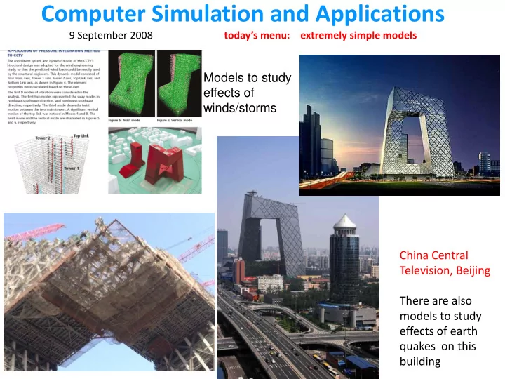
China Central Television, Beijing There are also models to study effects of earth quakes on this building Models to study effects of winds/storms

Practice yourself, for heaven’s sake, in little things, and thence proceed to greater. – Epictetus (Discourses IV, i) We will obey this adagium today. But don’t fret: what we are going to study today is rather indicative

• f the more general situations!

I will try to convey the ideas and intuition

predicitibility and reproducibility in science

Poincaré in ‘Science and Method’ (1903): “If we knew exactly the laws of nature and the situation of the universe at the initial moment, we could predict exactly the situation of that same universe at a succeeding moment. But even if it were the case that the natural laws had no longer any secret for us, we would still only know the initial situation approximately. If that enabled us to predict the succeeding situation with the same approximation, that is all we require, and we should say that the phenomenon had been predicted, that it is governed by laws. But it is not always so; it may happen that small differences in the initial conditions produce very great ones in the final phenomena. A small error in the former will produce an enormous error in the latter. Prediction becomes impossible, and we have the fortuitous phenomenon. “

Dynamical Systems

• Let us consider the following utterly simple

function: f(x) = 2x

• This can be viewed as a model for bacteria

growth: the rule expresses the fact that the population doubles every hour

• If the culture has 10,000 bacteria, then after

an hour there will be 20,000 bacteria, after two hours 40,000 bacteria etc

Dynamical Systems

• A dynamical system consists of a set of

possible states, together with a rule that determines the present states in terms of past states.

• In previous slide, we discussed a simple

dynamical systems whose states are population levels, that change with time under the rule: here the variable n stands for time and designates the population at time n.

xn+1 = f(xn) = 2 xn xn

Discussion of motivation for iterative maps

xn+1 = f(xn)

a) Discretization of differential equations b) Poincaré map c) Functions seen as models for describing population levels which change at discrete times (as in our example of bacteria growth) d) Newton-Raphson method for solving equations f(x) =0 e) And many more ....

(Deterministic) Dynamical Systems

• We require rule to be deterministic, i.e. we

can determine the present state (population, for example) uniquely from the past states.

• No randomness!
• Possible model for the price of gold as

function of time would be: predict today’s price to be yesterday’s plus or minus 1 euro, with the two possibilities equally likely.

• Instead of a dynamical system, this model

would be called random or stochastic process

Dynamical Systems

• Two types of dynamical systems:
• discrete time dynamical system

– Takes current state as input and updates the situation by producing a new state as output – State is whatever information which is needed in

• rder to be able to apply the rule

– aka(also known as): MAP

• continuous time dynamical system

– Essentially the limit of discrete systems with smaller and smaller updating times – Governing rule a set of differential equations

Aside: Recall why we study models

• Models suggest how real-world processes

behave

• Every model is at best an idealization. The goal

is to capture some feature of the physical process/system

• Today: we want to capture the patterns of

points on an orbit. We will find: sometimes simple, sometimes quite complicated (´chaotic´) even for simple maps

Aside: Recall why we study models

• The question to ask about a model is whether

the behavior it exhibits is because of its simplications or whether it captures the behavior despite the simplifications

• Modeling reality too closely may result in an

intractable model about which little can be learned

• Model building is an art (and a ´science´)

Aside: Recall why we study models

• Today we try to get a handle on possible

behaviors of maps by considering the simplest

• nes

• ne-dimensional Maps
• Recall we want to: Predict how a system will

evolve as time progresses

• Our first example, the population evolves by

single rule f(x) = 2x. The output of the rule is used as input value for the next hour, and the same doubling rule is applied again

• The evolution of this system is described by

the composition of the function f: given (initial value) we want to know for large k:

x0 x0, f (x0), f (f (x0)), , f (  f (f (x0))), 

k times Define: fk (x0) := f (  f (f (x0))), k times Orbit of x0

• ne-dimensional Maps
• Clearly for the example f(x) = 2x the

population will grow without bound (exponential growth)

• Malthus (1798): limits to growth
• Real habitats have finite resources

The (family) Logistic Map(s)

Improved model: f(x) = a x(1-x) introduced by Verhulst (1845) to simulate the growth in a closed area: The number of species xn+1 in the year n+1 is proportional to the number in the previous year xn and to the remaining area, which is diminished, propertionally, to xn where the parameter a depends on the fertility, the actual area of living etc. Name: LOGISTIC GROWTH MODEL

• (Aside: for our bacteria example x is measured in

millions)

The (family) Logistic Map(s)

Let us focus on the case where the paramater is 2: f(x) = 2 x(1-x)

Steady state

k f(x)=2x f(x)=2x(1-x) f(x)=2x(1-x) 0,01 0,01 0,9 1 0,02 0,0198 0,18 2 0,04 0,03881592 0,2952 3 0,08 0,074618489 0,41611392 4 0,16 0,13810114 0,485926251 5 0,32 0,23805843 0,499603859 6 0,64 0,362773228 0,499999686 7 1,28 0,462337626 0,5 8 2,56 0,497163091 0,5 9 5,12 0,499983904 0,5 10 10,24 0,499999999 0,5 11 20,48 0,5 0,5 12 40,96 0,5 0,5

Definitions

• A function whose domain(input) and

range(output space) are the same is called a map.

• Let x be a point and let f be a map. The orbit of

x under f is the set of points { f0(x) = x, f1(x) = f(x), f2(x) = f (f(x)), ... , fk(x) = f(fk-1(x)), ... }.

• The starting point x for the orbit is called the

initial value of the orbit.

• A point p is a fixed point of the map f, if f(p)=p

Example

• The function from the real line

to the real line is a map. Considered as from [0,1] to [0, 1] is another map.

• The orbit of x=0.01 under f is {0.01, 0.0198,

0.0388,...}

• The fixed points of f are x=0 and x=1/2.

f(x) = 2 x(1-x)

Graphically computing orbits: Cobweb Plots

x0 = 0.375 The line y=x, the diagonal, is an auxiliary “hulplijn” etcetera WHY do you get orbit? In words: Go from xo to the graph of the function, from the graph to the diagonal, from the diagonal to the graph, etc., etc. f(x) = 2x

Graphically computing orbits: Cobweb Plots

x0 = 0.375 (xo, x1)

Graphically computing orbits: Cobweb Plots

x0 = 0.375 (xo, x1) (?, x1)

Graphically computing orbits: Cobweb Plots

x0 = 0.375 (xo, x1) (?, x1) = (x1, x1)

Graphically computing orbits: Cobweb Plots

x0 = 0.375 (xo, x1) (x1, x1)

Graphically computing orbits: Cobweb Plots

x0 = 0.375 (xo, x1) (x1, x1) (?, 0)=(x1, 0)

Graphically computing orbits: Cobweb Plots

x0 = 0.375 (xo, x1) (x1, x1) (x1, x2)

Graphically computing orbits: Cobweb Plots

x0 = 0.375 (xo, x1) (x1, x1) (x1, x2) (?, x2)

Graphically computing orbits: Cobweb Plots

x0 = 0.375 (xo, x1) (x1, x1) (x1, x2) (?, x2) =(x2, x2)

Graphically computing orbits: Cobweb Plots

x0 = 0.375 (xo, x1) (x1, x1) (x1, x2) (x2, x2)

Graphically computing orbits: Cobweb Plots

x0 = 0.375 (xo, x1) (x1, x1) (x1, x2) (x2, x2) (x2, 0)

Graphically computing orbits: Cobweb Plots

x0 = 0.375 (xo, x1) (x1, x1) (x1, x2) (x2, x2) (x2, x3)

Graphically computing orbits: Cobweb Plots

x0 = 0.077 f(x) = 2x(1-x)

Plot of f(x) = (3 ¢ x – x3.0) / 2.0 Cobweb for initial values = 1.8 and 1.6

f(x)=1.0-1.4 x2

xo x1 x1 x2 x2 x3 x4

Stability of Fixed Points

• Very important point: if a fixed point (or

periodic point – defined later) is to be relevant for observations in the dyn. sys. described by f, then we need to know where it persists under small perturbations

• Why small perturbations?

Stability of Fixed Points

• We might consider different kinds of

perturbation

– Perturbation of the initial point: “do systems in nearby initial points evolve similarly? – Perturbations of the function f: “f is only approximately known” – Stochastic perturbations: “The true equation is not xn+1 = f(xn) but xn+1 = f(xn)+r(xn), where r(x) is a small variation of f(xn) with some a priori probability

Stability of Fixed Points

• f(x) = (3 ¢ x – x3.0) / 2.0 gave some insight into the

question of stability.

• The derivative of the map at the fixed point p is a

measure of how the distance between p and a nearby point is magnified or shrunk by f.

• 0 and 0.1 are 0.1 units apart, after applying the rule f

to both points, the distance separating the points is roughly f’(0). (value = 1.5)

• We want to call the fixed point 0 “unstable”when

points very near to 0 tend to move away from 0.

Stability of Fixed Points

The concept of “near” to a point p : all real numbers x which lie within a distance ε to p (notation Nε(p) ). Or more precise: let R denote the real numbers and p some real number, then

Nε(p) = { x in R : |x-p| < ε } Sometimes also calle the ε-neighborhood (epsilong- neighborhood) of p. We usually think of ε as a small, positive number.

Stability of Fixed Points: Definitions

• Let f be a map on R and let p be a real number such that

f(p)=p. If all points sufficiently close are attracted to p, then p is called a sink or an attracting fixed point.

• More precisely, if there is a ε > 0 such that for all x in the

epsilon-neigborhood Nε(p) : Limk  ∞ fk(x) = p, then p is a sink.

• If all points sufficiently close to p are repelled from p, the p is

called a source or a repelling fixed point.

• More precisely: if there is an epsilon-neighborhood Nε(p) such

that for each x in Nε(p) except p itself eventually maps

• utside of Nε(p), then p is a source.

Stability of Fixed Points: A Theorem

• Let f be a differentiable map on R and assume p is a fixed

point of f. Then: a) If |f’(p)| < 1, then p is a sink b) If |f’(p)| > 1, then p is a source

• Can readily proof this. The proof is instructive because we

learn from the proof what the rate of convergence is of fk(x) to p.

• Our definition of a fixed-point sink requires that the sink

attract some epsilon-neighborhood (p-ε, p+ε) of nearby points.

• According to the definition: ε could extremely small (although

nonzero).

• The set of points (=real numbers) x whose orbit converges to

the sink is called the basin of the sink).

• Sinks often attract orbits from a large set of initial points:
• For instance, f(x) = 2x (1-x):

a) Fixed points 0 and ½ b) f’(0) = 2 and f’(1/2)=0 c) Thus (see theorem of previous slide): 0 is a repellor and ½ is an attractor d) Basin of attraction of ½ is (0,1) (do this with a) cobweb and b) algebraically) e) (-∞,0) U (1,∞): each initial value in this set has an orbit that tends toward -∞

Stability of Fixed Points: BASINS

Stability of Fixed Points: BASINS

• What about f(x) = (3 ¢ x – x3.0) / 2.0 ?
• Fixed points? Classify fix points. Find the basins of the two
• sinks. (Already harder than previous example.)

Periodic Points

Periodic Orbits and Their Stability