Why Bayesian methods in Simulation? Simulation Simulation Model - - PowerPoint PPT Presentation

▶

Aug 21, 2022 261 likes •480 views

Outline Why Bayesian methods in Simulation? Simulation Simulation Model Inputs BAYESIAN IDEAS Output Random Simulated Statistical, pr FOR DISCRETE EVENT SIMULATION: Y r Numbers Variates Control,

SLIDE 1

Outline

BAYESIAN IDEAS FOR DISCRETE EVENT SIMULATION: WHY, WHAT AND HOW

Stephen E. Chick1

1Technology and Operations Management

INSEAD Fontainebleau, France

2006 Winter Simulation Conference

WSC’06 Bayesian Ideas for Simulation

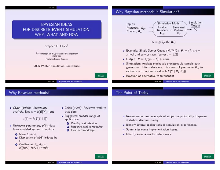
Why Bayesian methods in Simulation?

Inputs Statistical, θpr Control, θcr

✲ ✲ ✬ ✫ ✩ ✪

Simulation Model

✲ Random Numbers

Urij

✲ Simulated Variates Xrij ✲ ✲

Simulation Output Yr Yr = g(θp, θc; Ur) Example: Single Server Queue (M/M/1): θp = (λ, µi) = arrival and service rates (server i = 1, 2) Output: Y ≈ λ/(µi − λ) + noise Simulation: Analyze stochastic processes via sample path

generation. Inform decisions: pick control parameter θc, to

estimate or to optimize value h(E[Y | θp, θc]) Bayesian as alternative to frequentist

WSC’06 Bayesian Ideas for Simulation

Why Bayesian methods?

Glynn (1986): Uncertainty

analysis. Not α = h(E[Y ]), but

α(θ) = h(E[Y | θ]) Unknown parameters, p(θ), data from modeled system to update

Mean E[α(Θ)]

Distribution of α(Θ) induced by Θ

Credible set: θlo, θhi so p([h(θlo), h(θhi)]) = 95%

Chick (1997): Reviewed work to that date. Suggested broader range of application.

Ranking and selection

Response surface modeling

Experimental design

WSC’06 Bayesian Ideas for Simulation

The Point of Today

Review some basic concepts of subjective probability, Bayesian statistics, decision theory. Identify several applications to simulation experiments. Summarize some implementation issues. Identify some areas for future work.

WSC’06 Bayesian Ideas for Simulation

SLIDE 2

Related work

See the WSC (2006) paper and chapter in Henderson and Nelson book for a long (but incomplete) citation list for work over the last 10 years on: Formal Bayes or decision theoretic theory Applications: scheduling, insurance, finance, traffic modeling, public health, waterway safety, supply chain and other areas Bayes and deterministic simulations Favorite books on subjective and Bayesian probability and decision theory Public Policy and Health Economics: increasingly uses simulation (in addition to decision trees, Markov chains), and increasingly requires probabilistic sensitivity analysis.

WSC’06 Bayesian Ideas for Simulation Getting down To brass tacks Applications Implementation Summary What is Bayes? Prior Probability Asymptotic Theorems Dec

Outline

1 Getting down to brass tacks

Subjective and Bayesian methods Assessing prior probability Asymptotic Theorems Decisions, loss, and value of information Entropy and Kullback-Leibler Discrepancy

2 Applications

Uncertainty Analysis Selecting from Multiple Candidate Distributions Selecting the Best System Metamodels

3 Implementation 4 Summary

WSC’06 Bayesian Ideas for Simulation Getting down To brass tacks Applications Implementation Summary What is Bayes? Prior Probability Asymptotic Theorems Decisi

Getting down to brass tacks

Probability of 7 heads in the first 10 flips? How to approach the problem. . .

WSC’06 Bayesian Ideas for Simulation Getting down To brass tacks Applications Implementation Summary What is Bayes? Prior Probability Asymptotic Theorems Dec

Getting down to brass tacks

Probability of 7 heads in the first 10 flips? Comte d’Alembert (18th cent.) Indifference says maybe 1/11? But wait, for one flip, probability of heads is 1/2? See Savage (1972) and Kreps (1988).

WSC’06 Bayesian Ideas for Simulation

SLIDE 3

Getting down To brass tacks Applications Implementation Summary What is Bayes? Prior Probability Asymptotic Theorems Decisi

Getting down to brass tacks

Probability of 7 heads in the first 10 flips? Dwight (an unreconstructed frequentist)

10! 7!3!θ7(1 − θ)3, where θ = limn→∞ X1+...+Xn n

(a.e.). If we rent Madison Square garden and flip the tack repeatedly, I can estimate θ for you. What confidence and how accurately do you need to know θ?

Hmmm. . .

WSC’06 Bayesian Ideas for Simulation Getting down To brass tacks Applications Implementation Summary What is Bayes? Prior Probability Asymptotic Theorems Dec

Getting down to brass tacks

Probability of 7 heads in the first 10 flips? Dwight (an unreconstructed frequentist)

10! 7!3!θ7(1 − θ)3, where θ = limn→∞ X1+...+Xn n

(a.e.). If we rent Madison Square garden and flip the tack repeatedly, I can estimate θ for you. What confidence and how accurately do you need to know θ? Let’s reformulate the question . . .

WSC’06 Bayesian Ideas for Simulation Getting down To brass tacks Applications Implementation Summary What is Bayes? Prior Probability Asymptotic Theorems Decisi

Why am I a Bayesian?

Will you accept the following bet now? You get $100 if there are 7 heads, but you pay $5 if not. more from Dwight I can’t answer until I have a good idea of what θ is. Guessing wouldn’t be scientific.

WSC’06 Bayesian Ideas for Simulation Getting down To brass tacks Applications Implementation Summary What is Bayes? Prior Probability Asymptotic Theorems Dec

Why am I a Bayesian?

Ralph Probability of 7 heads in the first 10 flips? I’m willing to use probability for personal judgments 1

10! 7!3!θ7(1 − θ)3π(θ)dθ, where π(θ) is a prior probability.

I’ll update with Bayes’ rule, to get posterior probability p(θ | xn) = π(θ)p(xn | θ) p(xn) = π(θ) n

i=1 p(xi | θ)

p(xn | θ)dπ(θ)

WSC’06 Bayesian Ideas for Simulation

SLIDE 4

Getting down To brass tacks Applications Implementation Summary What is Bayes? Prior Probability Asymptotic Theorems Decisi

Why am I a Bayesian?

Lenny Probability of 7 heads in the first 10 flips? Fair bets: I set p(E1) > p(E2) if I prefer the first bet: 1)

2)
Exchangeability (weaker than i.i.d.)

p(x1, x2, . . . , xn) = p(xs1, xs2, . . . , xsn) for permutations s on {1, 2, . . . , n} for arbitrary n.

WSC’06 Bayesian Ideas for Simulation Getting down To brass tacks Applications Implementation Summary What is Bayes? Prior Probability Asymptotic Theorems Dec

Why am I a Bayesian?

Lenny Exchangeability plus conceptually infinite N imply limN→∞ p(7 heads in first 10 flips) = 1

10! 7!3!θ7(1 − θ)3dF(θ)

de Finetti (1990)-like representation Ralph assumed conditional i.i.d., while Lenny derives formula from exchangeability Probability defined by bet preferences, not repeated outcomes

WSC’06 Bayesian Ideas for Simulation Getting down To brass tacks Applications Implementation Summary What is Bayes? Prior Probability Asymptotic Theorems Decisi

Implication for Simulation: Yr = g(θp, θe, θc; Ur)

Inputs Statistical, θpr Control, θcr Environmental, θer

✲ ✲ ✲ ✬ ✫ ✩ ✪

Simulation Model

✲ Random Numbers

Urij

✲ Simulated Variates Xrij ✲ ✲

Simulation Output Yr Input selection: Infinite exchangeable sequence Xij from modeled system to infer ith statistical input, θpi

WSC’06 Bayesian Ideas for Simulation Getting down To brass tacks Applications Implementation Summary What is Bayes? Prior Probability Asymptotic Theorems Dec

Implication for Simulation: Yr = g(θp, θe, θc; Ur)

Inputs Statistical, θpr Control, θcr Environmental, θer

✲ ✲ ✲

Inputs Statistical, θp Control, θc Environmental, θe

✲ ✲ ✲ ✬ ✫ ✩ ✪

Simulation Model

✲ Random Numbers

Urij

✲ Simulated Variates Xrij ✲ ✻ ✬ ✫ ✩ ✪

Metamodel

✲ Metamodel Parameters

Ψ

✲ ✲

Simulation Output Yr

✲

Metamodel Output Y Input selection: Infinite exchangeable sequence Xij from modeled system to infer ith statistical input, θpi Metamodeling: Infinite exchangeable Yr to infer Ψ.

WSC’06 Bayesian Ideas for Simulation

SLIDE 5

Getting down To brass tacks Applications Implementation Summary What is Bayes? Prior Probability Asymptotic Theorems Decisi

Part of the process

Establish exchangeability arguments, posit potential likelihood functions for observables, given unknown quantities Assess prior distributions for unknown quantities Relevant asymptotic theorems Decisions, loss, and value of information

ranking and selection,

ther experimental design issues

WSC’06 Bayesian Ideas for Simulation Getting down To brass tacks Applications Implementation Summary What is Bayes? Prior Probability Asymptotic Theorems Dec

Outline

1 Getting down to brass tacks

Subjective and Bayesian methods Assessing prior probability Asymptotic Theorems Decisions, loss, and value of information Entropy and Kullback-Leibler Discrepancy

2 Applications

Uncertainty Analysis Selecting from Multiple Candidate Distributions Selecting the Best System Metamodels

3 Implementation 4 Summary

WSC’06 Bayesian Ideas for Simulation Getting down To brass tacks Applications Implementation Summary What is Bayes? Prior Probability Asymptotic Theorems Decisi

Subjective Methods

We need a prior distribution for unknown parameters. For a Bernoulli outcome . . . de Finetti (1990), Savage (1972) require You to assess your personal belief, π(θ) to describe p(Θ ≤ θ) Important gain in flexibility Consistent with expected value decision theory Kahneman, Slovic, and Tversky (1982) describe difficulties with elicitation . . . Some seek ‘automated’ methods . . .

WSC’06 Bayesian Ideas for Simulation Getting down To brass tacks Applications Implementation Summary What is Bayes? Prior Probability Asymptotic Theorems Dec

Principle of Indifference

For finite exchangeable sequence, set θN = X1+...+XN

N

∈ {0/N, 1/N, . . . , (N − 1)/N, 1} Indifference: discrete uniform for finite N Limit: limN→∞ p(θN) D → uniform[0, 1] Laplace (1812) used uniform[0, 1] for his prior probability that the sun would come up tomorrow Coordinate dependence for continuous r.v. (Xi versus log Xi)

WSC’06 Bayesian Ideas for Simulation

SLIDE 6

Getting down To brass tacks Applications Implementation Summary What is Bayes? Prior Probability Asymptotic Theorems Decisi

Jeffrey’s invariant prior

π(θ) ∝ |H(θ)|1/2dθ, where H is the expected information in

ne observation,

H(θ) = EX

−∂2log p(X | θ)

∂θ2

(1) ‘uniform’ with respect to the natural metric induced by the likelihood function (Kass 1989) Jeffreys’ prior for Bernoulli sampling is beta(1/2, 1/2) For some likelihoods, Jeffreys’ prior is improper (doesn’t integrate to 1). Might be used formally

WSC’06 Bayesian Ideas for Simulation Getting down To brass tacks Applications Implementation Summary What is Bayes? Prior Probability Asymptotic Theorems Dec

Conjugate prior distribution

Bernoulli sampling Set sn = n

i=1 xi

Likelihood: p(xn|θ) ∝ θsn(1 − θ)n−sn Prior: π(θ) ∝ θα−1(1 − θ)β−1, a beta(α, β) distribution Posterior: ∝ θα+sn−1(1−θ)β+n−sn−1, a beta(α + sn, β + n − sn) (conjugate) distribution Exponential family Likelihood: p(x | θ) = a(x)h0(θ) exp d

j=1 cjφj(θ)hj(x)

Canonical conjugate prior: p(θ) =

K(t)[h0(θ)]n0 exp d

j=1 cjφj(θ)tj

Posterior, given n data points: has

parameters n0 + n and sum of t = (t1, t2, . . . , td) and sufficient statistics (Bernardo and Smith 1994)

WSC’06 Bayesian Ideas for Simulation Getting down To brass tacks Applications Implementation Summary What is Bayes? Prior Probability Asymptotic Theorems Decisi

‘Noninformative’

The uniform[0, 1] distribution is conjugate for Bernoulli sampling—a beta(1, 1) distribution. ‘Noninformative’ means ‘evenly spread’—a heuristic term For canonical conjugate prior (for exponential family), the posterior has parameter n0 + n Some think of n0 + n as an ‘effective’ number of data points ‘Noninformative’ associated with a small n0 Others Jaynes (1983): maximum entropy methods Berger (1994), Kass and Wasserman (1996): Default rules Useful? Actually informative?

WSC’06 Bayesian Ideas for Simulation Getting down To brass tacks Applications Implementation Summary What is Bayes? Prior Probability Asymptotic Theorems Dec

Outline

1 Getting down to brass tacks

Subjective and Bayesian methods Assessing prior probability Asymptotic Theorems Decisions, loss, and value of information Entropy and Kullback-Leibler Discrepancy

2 Applications

Uncertainty Analysis Selecting from Multiple Candidate Distributions Selecting the Best System Metamodels

3 Implementation 4 Summary

WSC’06 Bayesian Ideas for Simulation

SLIDE 7

Getting down To brass tacks Applications Implementation Summary What is Bayes? Prior Probability Asymptotic Theorems Decisi

Classic Analogs for Infinite Exchangeable Sequences

Classical asymptotic theorems (e.g. Billingsley 1986) . . . laws of large numbers (LLN) central limit theorem (CLT) law of iterated logarithm (LIL) . . . have Bayesian interpretations if considered conditional on mean and standard deviation of an infinite exchangeable sequence.

WSC’06 Bayesian Ideas for Simulation Getting down To brass tacks Applications Implementation Summary What is Bayes? Prior Probability Asymptotic Theorems Dec

Bayesian LLN

A Bayesian extension of the LLN allows for sample averages to converge to random variables rather than to ‘true’ means. Theorem (Bayesian LLN) If ¯ Xn and ¯ Ym are respectively the averages of n and m exchangeable random quantities Xi (the two averages may or may not have some terms in common), the probability that

Xn − ¯ Ym

> ǫ

may be made arbitrarily small by taking n and m sufficiently large (de Finetti 1990, p. 216 assumes a finite variance).

WSC’06 Bayesian Ideas for Simulation Getting down To brass tacks Applications Implementation Summary What is Bayes? Prior Probability Asymptotic Theorems Decisi

Theorem (Posterior Normality) For each n, let pn(·) be the posterior pdf of the d-dimensional parameter θn given xn = (x1, . . . , xn), let ˜ θn be its mode (MAP), and define the d × d Bayesian observed information matrix Σ−1

n

by Σ−1

n

= −∂2log pn(θ | xn) ∂θ2

θn

. (2) Then φn = Σ−1/2

n

(θn − ˜ θn) converges in distribution to a standard (multivariate) normal random variable (Bernardo and Smith 1994, Prop 5.14 needs regularity conditions). Frequentist analog: asserts that MLE is asymptotically normally distributed about a ‘true’ θ0 (Law and Kelton 2000), as opposed to describing uncertainty about θ.

WSC’06 Bayesian Ideas for Simulation Getting down To brass tacks Applications Implementation Summary What is Bayes? Prior Probability Asymptotic Theorems Dec

Outline

1 Getting down to brass tacks

Subjective and Bayesian methods Assessing prior probability Asymptotic Theorems Decisions, loss, and value of information Entropy and Kullback-Leibler Discrepancy

2 Applications

Uncertainty Analysis Selecting from Multiple Candidate Distributions Selecting the Best System Metamodels

3 Implementation 4 Summary

WSC’06 Bayesian Ideas for Simulation

SLIDE 8

Getting down To brass tacks Applications Implementation Summary What is Bayes? Prior Probability Asymptotic Theorems Decisi

Decisions under uncertainty

Uncertainty described by probability ⇒ modeler can assess expected value of information (EVI) of additional data. EVI is useful in experimental design. EVI : value of resolving uncertainty with respect to a loss function L(d, ω) that describes losses when a decision d is chosen when the state of nature is ω. Data from experiment can reduce uncertainty about ω, reduce expected loss.

WSC’06 Bayesian Ideas for Simulation Getting down To brass tacks Applications Implementation Summary What is Bayes? Prior Probability Asymptotic Theorems Dec

Example: What is the mean? Setup

Example adapted from de Groot (1970) illustrates key concepts used for VIP procedures (Chick and Inoue 2001b) Decide if unknown mean W of normal distribution (known σ2) is smaller (decision d = 1) or larger (d = 2) than w0. Exchangeable samples Xn = (X1, X2, . . . , Xn), with p(Xi) ∼ Normal

w, σ2

, given W = w, are available Goal: design experiment (choose n) to balance sampling cost (cn) and expected opportunity cost if wrong answer chosen L (1, w) =

if w ≤ w0

w − w0 if w > w0, L (2, w) = w0 − w if w ≤ w0 if w > w0.

WSC’06 Bayesian Ideas for Simulation Getting down To brass tacks Applications Implementation Summary What is Bayes? Prior Probability Asymptotic Theorems Decisi

Example: What is the mean? If we knew. . .

Prior: W ∼ Normal (µ, 1/τ) is conjugate. NOTE: τ is the precision in our uncertainty about unknown mean, W . Posterior: Observing Xn = xn would result in p(w | xn) ∼ Normal

z, τ −1

n

= posterior mean of W = E[W | xn] = τµ + n

σ2 ¯

xn τ + n

σ2

τn = posterior precision of W = τ + n/σ2. τ −1

n

equals the asymptotic posterior variance approximation Σn from theorem

WSC’06 Bayesian Ideas for Simulation Getting down To brass tacks Applications Implementation Summary What is Bayes? Prior Probability Asymptotic Theorems Dec

Example: What is the mean? How much to know. . .

Posterior mean z for unknown w influences the decision, but depends upon n, which is selected before Xn is seen. Conditional distribution of ¯ Xn given w is Normal

w, σ2/n
Predictive distribution p(z) of the posterior mean

Z = E[W | Xn] = (τµ + n

σ2 ¯

Xn)/τn Mixing over prior π(w) implies a predictive distribution Z ∼ Normal

µ, τ −1

z

= τ(τ + n/σ2)/(n/σ2) Note: τ −1

z

→ 0 when n → 0 (no new information). If n → ∞, then Var[Z] → σ2.

WSC’06 Bayesian Ideas for Simulation

SLIDE 9

Getting down To brass tacks Applications Implementation Summary What is Bayes? Prior Probability Asymptotic Theorems Decisi

Example: What is the mean? What is the risk. . .

To minimize risk (sampling cost + expected loss from potentially incorrect decision), pick n to minimizes a nested expectation ρ(n) = cn + EXn[EW [L(d(Xn), W ) | Xn]]. General technique: set L∗(d, w) = L(d, w) − L(1, w), which is 0 if d = 1 and is w0 − w if d = 2. Then EW [L∗(d(Xn), W ) | Xn] =

if d = 1

w0 − Z if d = 2. (3) To minimize loss in Eq. 3, assert d(Xn) = 2 (‘bigger’) if posterior mean exceeds threshold, Z > w0, and assert d(Xn) = 1 (‘smaller’) if Z ≤ w0.

WSC’06 Bayesian Ideas for Simulation Getting down To brass tacks Applications Implementation Summary What is Bayes? Prior Probability Asymptotic Theorems Dec

Example: What is the mean? Expected loss

Decision depends on Xn via Z; Z has normal distribution Expected loss found with standard normal loss for newsboy LN[s] =

(t − s)φ(t)dt = φ(s) − s(1 − Φ(s)) E[L∗(d(Xn), W )] = EXn[EW [L∗(d(Xn), W ) | Xn]] = −τ

−1 2

z

LN[τ

1 2

z (w0 − µ)]

Add back E[L(1, W )], use prior for W E[L(d(Xn), W )] = τ

−1 2 LN[τ 1 2 (w0 − µ)] − τ −1 2

z

LN[τ

1 2

z (w0 − µ)]

EVI and EVPI

WSC’06 Bayesian Ideas for Simulation Getting down To brass tacks Applications Implementation Summary What is Bayes? Prior Probability Asymptotic Theorems Decisi

Example: What is the mean? What is the risk. . .

First-order optimality condition ∂ρ ∂n = 1 2τ

− 3

z

φ[τ

1 2

z (w0 − µ)] · −τ 2σ2

n2 + c = 0 For small costs c → 0, the sample size is large. Since τz → τ as n → ∞, the optimal sample size n is asymptotically n∗ ≈

1 2 σ2φ[τ 1 2

z (w0 − µ)]/(2c)

1/2 . Asymptotic approximations are a second useful tool to identify criteria-based sampling plans. Extensions of these ideas used to derive VIP procedures (Chick and Inoue 2001b).

WSC’06 Bayesian Ideas for Simulation Getting down To brass tacks Applications Implementation Summary What is Bayes? Prior Probability Asymptotic Theorems Dec

Alternate approximation

Regular exponential family: asymptotic variance approximation Σn from theorem simplifies to H−1(θ)/(n0 + n), where H is the expected information from one observation (Eq. 1), if canonical conjugate prior distribution is used Approximate effect of m new samples is to change posterior to Normal

θn, Σn n0 + n n0 + n + m

Used for OCBA (Chen 1996), sampling plans for field data (Ng and Chick 2001). Frequentist result to obtain CI of desired size (Law and Kelton 2000)

WSC’06 Bayesian Ideas for Simulation

SLIDE 10

Getting down To brass tacks Applications Implementation Summary What is Bayes? Prior Probability Asymptotic Theorems Decisi

Outline

1 Getting down to brass tacks

Subjective and Bayesian methods Assessing prior probability Asymptotic Theorems Decisions, loss, and value of information Entropy and Kullback-Leibler Discrepancy

2 Applications

Uncertainty Analysis Selecting from Multiple Candidate Distributions Selecting the Best System Metamodels

3 Implementation 4 Summary

WSC’06 Bayesian Ideas for Simulation Getting down To brass tacks Applications Implementation Summary What is Bayes? Prior Probability Asymptotic Theorems Dec

Another loss function: discrepancy

Kullback-Leibler discrepancy: difference between distributions Discrete distributions ˜ p and p, δ(p || ˜ p) =

pi log(˜ pi/qi). Continuous r.v. X with densities ˜ f and fθ = f (x | θ), δ(fθ || ˜ f ) =

f (x) log ˜ f (x) f (x | θ)dx. One use: loss function for eliciting probability. If you believe the distribution is ˜ f , and you lose δ(f || ˜ f ) if you provide a distribution f , then you should honestly report ˜ f (Bernardo 1979)

WSC’06 Bayesian Ideas for Simulation Getting down To brass tacks Applications Implementation Summary What is Bayes? Prior Probability Asymptotic Theorems Decisi

Discrepancy: Other uses

Select design matrix dΘ of r vectors of inputs (θpi, θei, θci) for i = 1, 2, . . . , r with output Y in order to best differentiate the posterior distribution of the response parameters ψ from the prior distribution for ψ (Bayesian D-optimal, Bernardo 1979; Smith and Verdinelli 1980; Ng and Chick 2004)

p(Y | dΘ)
p(ψ | Y) log p(ψ | Y)

p(ψ) dψ

Select maximum entropy prior distribution (Jaynes 1983) More later: input distribution selection . . .

WSC’06 Bayesian Ideas for Simulation Getting down To brass tacks Applications Implementation Summary Uncertainty Analysis Input Distribution Selection Ranking/Selec

Outline

1 Getting down to brass tacks

Subjective and Bayesian methods Assessing prior probability Asymptotic Theorems Decisions, loss, and value of information Entropy and Kullback-Leibler Discrepancy

2 Applications

Uncertainty Analysis Selecting from Multiple Candidate Distributions Selecting the Best System Metamodels

3 Implementation 4 Summary

WSC’06 Bayesian Ideas for Simulation

SLIDE 11

Getting down To brass tacks Applications Implementation Summary Uncertainty Analysis Input Distribution Selection Ranking/Selec

Why Uncertainty Analysis?

Simple Example µj → Simulation → Yj = 2µj + ej Input model: Xℓ ∼ Normal

µ, σ2

x

, known σ2

x

Data: Xℓ observed (ℓ = 1, 2, . . . , n0) Run r replications with ¯ Xn0 input for µ Construct 90% CI: ¯ Yr ± z0.95

ˆ σy √r

Coverage?

If µ is known, expect coverage to be 90%. But µ is not known.

WSC’06 Bayesian Ideas for Simulation Getting down To brass tacks Applications Implementation Summary Uncertainty Analysis Input Distribution Selection Ranking/Selec

Why Uncertainty Analysis?

Simple Example µj → Simulation → Yj = 2µj + ej Input model: Xℓ ∼ Normal

µ, σ2

x

, known σ2

x

Data: Xℓ observed (ℓ = 1, 2, . . . , n0) Run r replications with ¯ Xn0 input for µ Construct 90% CI: ¯ Yr ± z0.95

ˆ σy √r

Coverage?

If µ is known, expect coverage to be 90%. But µ is not known. CI can be meaningless (several authors. . . )

WSC’06 Bayesian Ideas for Simulation Getting down To brass tacks Applications Implementation Summary Uncertainty Analysis Input Distribution Selection Ranking/Selec

Why Uncertainty Analysis?

Simple Example µj → Simulation → Yj = 2µj + ej Input model: Xℓ ∼ Normal

µ, σ2

x

, known σ2

x

Data: Xℓ observed (ℓ = 1, 2, . . . , n0) Run r replications with ¯ Xn0 input for µ Construct 90% CI: ¯ Yr ± z0.95

ˆ σy √r

√Vtot

Account for parameter uncertainty Vtot =

σ2

r + 4σ2

n0 , so try ¯

Yr ± z0.95 √Vtot

WSC’06 Bayesian Ideas for Simulation Getting down To brass tacks Applications Implementation Summary Uncertainty Analysis Input Distribution Selection Ranking/Selec

Why Uncertainty Analysis?

Simple Example µj → Simulation → Yj = 2µj + ej Input model: Xℓ ∼ Normal

µ, σ2

x

, known σ2

x

Data: Xℓ observed (ℓ = 1, 2, . . . , n0) Run r replications with ¯ Xn0 input for µ Construct 90% CI: ¯ Yr ± z0.95

ˆ σy √r

√Vtot

For known mean response g, input parameters θ = (θ1, . . . , θk) Vtot ≈

σ2

r + k i=1

βiH(˜

θi)−1β

T i

ni

where gradient βi = ∂g(˜ θ)T

∂θi

θ (asymptotics. Cheng & Holland; Ng & Chick; Wilson & Zouaoui)

WSC’06 Bayesian Ideas for Simulation

SLIDE 12

Getting down To brass tacks Applications Implementation Summary Uncertainty Analysis Input Distribution Selection Ranking/Selec

Why Uncertainty Analysis? Estimate response

Inputs θ1 = (µ1, λ1) θ2 = (µ2, λ2) θ3 = (µ3, λ3)

✲ ✲ ✲ ✬ ✫ ✩ ✪

Simulation

✲

Yr = g(θ) + σZ = β0 + k

i=1 β2i−1µi + β2iλi

+β7µ1µ2 + β8µ2

1 + σZ

Assess Xiℓ ∼ Normal

µi, λ−1

i

for ith source of randomness

Observe data Xiℓ are observed (i = 1, 2, 3; ℓ = 1, 2, . . . , ni) Estimate unknown β with r0 runs (e.g. CCD from DOE) Vtot = ˆ σ2

y

r0 +

k

∂g(˜ θn, ˜ βr0) ∂θi Σni ∂g(˜ θn, ˜ βr0)T ∂θi

Vpar=O(n−1

)

+ Σβ ⊗ Σθ

Vresp=O(n−1

r−1)

WSC’06 Bayesian Ideas for Simulation Getting down To brass tacks Applications Implementation Summary Uncertainty Analysis Input Distribution Selection Ranking/Selec

Uncertainty Analysis: Uncertainty Reduction

Goal: Reduce uncertainty, not just quantify

r more replications mi more samples from source of randomness i

Optimization: min

r,mi

ˆ σ2

y

r0 + r +

k

ξi ni + mi + ζi (r0 + r)(ni + mi) r, mi ≥ CI Coverage (Ng and Chick 2006)

1000 2000 3000 4000 0.2 0.4 0.6 0.8 1

Coverage (target 95%) CI with Vtot

n0=20 n0=40 n0=60 n0=80 1000 2000 3000 4000 1 2 3 4 5 6

Half Width

n0=20 n0=40 n0=60 n0=80 1000 2000 3000 4000 0.2 0.4 0.6 0.8 1

CI with Vstoch Budget, B

n0=20 n0=40 n0=60 n0=80 1000 2000 3000 4000 0.005 0.01 0.015 0.02 0.025 0.03

Budget, B

n0=20 n0=40 n0=60 n0=80

WSC’06 Bayesian Ideas for Simulation Getting down To brass tacks Applications Implementation Summary Uncertainty Analysis Input Distribution Selection Ranking/Selec

Uncertainty Analysis

Sensitivity analysis: E[g(θ)] as a function of θ (average out stochastic uncertainty from u) Uncertainty analysis: E[Y | E], with both stochastic and parameter uncertainty, given all information E Bayesian Model Average (BMA) estimates EY [Y | E] for r = 1, . . . , R replications sample parameter θr ∼ p(θ | E) for i = 1, 2, . . . , n generate output yri given input θr end loop end loop Generate estimate ¯ y = R

r=1 1 R

n

i=1 yri n .

WSC’06 Bayesian Ideas for Simulation Getting down To brass tacks Applications Implementation Summary Uncertainty Analysis Input Distribution Selection Ranking/Selec

Variations on Estimating E[Y | E]

Zouaoui and Wilson (2003): decouple stochastic, parameter uncertainty; update estimate as new data becomes available with variations on BMA Andrad´

ttir and Glynn (2004): biased estimates of E[Y | θ];

quasi-random numbers; quadrature to select inputs θi Estimate distribution of conditional expectation E[Y | Θ, E]. Steckley and Henderson (2003) derive asymptotically optimal ways selecting r and n in BMA to produce a kernel density estimator (some conditions apply)

WSC’06 Bayesian Ideas for Simulation

SLIDE 13

Getting down To brass tacks Applications Implementation Summary Uncertainty Analysis Input Distribution Selection Ranking/Selec

Outline

1 Getting down to brass tacks

Subjective and Bayesian methods Assessing prior probability Asymptotic Theorems Decisions, loss, and value of information Entropy and Kullback-Leibler Discrepancy

2 Applications

Uncertainty Analysis Selecting from Multiple Candidate Distributions Selecting the Best System Metamodels

3 Implementation 4 Summary

WSC’06 Bayesian Ideas for Simulation Getting down To brass tacks Applications Implementation Summary Uncertainty Analysis Input Distribution Selection Ranking/Selec

Basic Problem

Which distribution/parameter to pick? ‘Usual’:

Pick q candidate input distributions (e.g. exponential, gamma, Weibull, lognormal)

Find MLE ˆ θi for candidates i = 1, . . . , q

Goodness-of-fit (χ-squared, K-S, A-D) tests

Concerns:

CI coverage if MLE/best distribution selected

How to select among unrejected models? . . . (Lindley 1957; Berger and Pericchi 1996)

WSC’06 Bayesian Ideas for Simulation Getting down To brass tacks Applications Implementation Summary Uncertainty Analysis Input Distribution Selection Ranking/Selec

Bayesian Input Selection

BMA applies without change for q candidates

Put prior on (M = m, θm), where m ∈ {1, 2, . . . , q}

Compute posterior p(m, Θm|E), sample from it in BMA

Chick (2001): stochastic process simulation context; moment matching method for commensurate prior distributions Zouaoui and Wilson (2004): decouple stochastic uncertainty from two types of structural uncertainty (candidate model & parameters); variance reduction for BMA; numerical analysis Model selected closest to the true model in sense of Kullback-Leibler divergence (Berk 1966; Bernardo and Smith 1994; Dmochowski 1999).

WSC’06 Bayesian Ideas for Simulation Getting down To brass tacks Applications Implementation Summary Uncertainty Analysis Input Distribution Selection Ranking/Selec

Outline

1 Getting down to brass tacks

Subjective and Bayesian methods Assessing prior probability Asymptotic Theorems Decisions, loss, and value of information Entropy and Kullback-Leibler Discrepancy

2 Applications

Uncertainty Analysis Selecting from Multiple Candidate Distributions Selecting the Best System Metamodels

3 Implementation 4 Summary

WSC’06 Bayesian Ideas for Simulation

SLIDE 14

Getting down To brass tacks Applications Implementation Summary Uncertainty Analysis Input Distribution Selection Ranking/Selec

Ranking and selection procedures differ?

What is it for?

Select the ‘best’ of a finite set Best identified by mean simulation response

What are the approaches?

IZ, Indifference zone: P(CS) ≥ 1 − α, δ∗, repeated applications of procedure VIP, Bayesian value of information procedures: Like selection of mean bigger or smaller than threshold, Bayesian inference, loss, EVI OCBA, Chen et al.: Heuristic, allocates samples to improve Bayesian PCS using ‘thought experiment’ σ2/r0 → σ2/(r0 + r)

Economic. Chick and Gans (2005) propose a new economic

approach, includes costs of replications and discounting, maximizes E[NPV] of decisions with simulation.

WSC’06 Bayesian Ideas for Simulation Getting down To brass tacks Applications Implementation Summary Uncertainty Analysis Input Distribution Selection Ranking/Selec

VIP procedures

Motivated by ‘statistical conservativeness’ of IZ approaches Two-stage: Unknown means of several systems.

Opportunity cost and 0-1 loss (P(CS)) Variances also unknown, different (conjugate prior, student marginal for mean) Optimal solution unknown except special cases Asymptotic approximation, Bonferroni bound for loss

Sequential:

In theory, should improve things Behrens-Fisher Seems to work quite well

WSC’06 Bayesian Ideas for Simulation Getting down To brass tacks Applications Implementation Summary Uncertainty Analysis Input Distribution Selection Ranking/Selec

Procedure LL(B), for opportunity cost (linear loss)

1 Specify the first-stage sample size r0. Take independent

replications yi1, . . . , yir0, for each system, i = 1, . . . , k

2 Compute all first-stage sample means ¯

xi = r0

i=1 yij/r0 and

sample variances ˆ σ2

i = Pr0

j=1(yij−¯

xi)2 r0−1

, order statistics ¯ x[1] ≤ . . . ≤ ¯ x[k], and λi,k = r0/(ˆ σ2

[k] + ˆ

σ2

[i])

3 If sampling budget is B, run ri more independent replications,

r[i] = B +

j∈S r0cj

j∈S
cjc[i]ˆ

σ2

j ηj

ˆ σ2

[i]η[i]

1/2 − r0 η[i] = (λi,k)1/2 (r0−1)+λi,k(¯

x[k]−¯ x[i])2 (r0−1)−1

φr0−1[(λi,k)1/2(¯ x[k] − ¯ x[i])] if [i] = [k] and η[k] = k−1

j=1 η[j]

4 Select system with largest ¯

¯ xi = r0+ri

j=1 yij/(r0 + ri)

WSC’06 Bayesian Ideas for Simulation Getting down To brass tacks Applications Implementation Summary Uncertainty Analysis Input Distribution Selection Ranking/Selec

Sample Comparison with Combined Procedure, C (MDM)

Figure Number of systems, k

f merit

Proc. 2 5 10 100 ANR All 738 3,429 8,784 42,862 Empirical C 0.8363 0.9140 0.9323 0.9763 P(CS) 0-1(B) 0.8527∗ 0.9117 0.9480∗ 0.9937∗ LL(B) 0.8500 0.9293∗ 0.9660∗ 0.9987∗ Empirical C 1.0000 0.9943 0.9990 1.0000

frac. ‘good’

0-1(B) 1.0000 0.9953 0.9977 0.9997 selections LL(B) 1.0000 0.9953 0.9993 1.0000 Expected C 0.8336 0.8379 0.8649 0.9318 posterior 0-1(B) 0.8446∗ 0.8339 0.8821∗ 0.9717∗ PCS LL(B) 0.8470∗ 0.8462∗ 0.9022∗ 0.9842∗ Expected C 0.0176 0.0138 0.0104 0.0037 bound, 0-1(B) 0.0157∗ 0.0128∗ 0.0075∗ 0.0012∗

pp. cost

LL(B) 0.0154∗ 0.0110∗ 0.0055∗ 0.0005∗ Monotone decreasing means (MDM). ∗ indicates statistically significant difference

WSC’06 Bayesian Ideas for Simulation

SLIDE 15

Getting down To brass tacks Applications Implementation Summary Uncertainty Analysis Input Distribution Selection Ranking/Selec

VIP: Common Random Numbers

Common random numbers (CRN) can sharpen contrasts between systems (e.g. same simulated demand pattern) Two-stage with screening (Chick and Inoue 2001a)

Run subset of systems in stage 2 Use ‘missing data’ formulas to update Select from even screened systems

Matrix intensive, heuristic provided Stage 1 1 2 3 4 5 . . . k

WSC’06 Bayesian Ideas for Simulation Getting down To brass tacks Applications Implementation Summary Uncertainty Analysis Input Distribution Selection Ranking/Selec

VIP: Common Random Numbers

Common random numbers (CRN) can sharpen contrasts between systems (e.g. same simulated demand pattern) Two-stage with screening (Chick and Inoue 2001a)

Run subset of systems in stage 2 Use ‘missing data’ formulas to update Select from even screened systems

Matrix intensive, heuristic provided Stage 1 Stage 2 1 2 3 4 5 . . . k

WSC’06 Bayesian Ideas for Simulation Getting down To brass tacks Applications Implementation Summary Uncertainty Analysis Input Distribution Selection Ranking/Selec

VIP: Common Random Numbers

Common random numbers (CRN) can sharpen contrasts between systems (e.g. same simulated demand pattern) Two-stage with screening (Chick and Inoue 2001a)

Run subset of systems in stage 2 Use ‘missing data’ formulas to update Select from even screened systems

Matrix intensive, heuristic provided Stage 1 Stage 2 Infer 1 2 3 4 5 . . . k

WSC’06 Bayesian Ideas for Simulation Getting down To brass tacks Applications Implementation Summary Uncertainty Analysis Input Distribution Selection Ranking/Selec

Summaries

VIP procedures have solid basis, perform numerically quite well Chick and Inoue (2001, 2001a, 2002).

Matlab: All procedures (0-1 or opportunity cost loss; two-stage

r independent sequential; two-stage CRN)

C: Independent replications, two-stage or sequential, both loss functions, plus variants (work in progress) to achieve Bayesian predictive targets for PCS and EOC

Can show asymptotic relation between certain VIP and OCBA procedures Specific Bayesian procedures with new stopping rules highly effective (Branke, Chick, and Schmidt 2005)

WSC’06 Bayesian Ideas for Simulation

SLIDE 16

Getting down To brass tacks Applications Implementation Summary Uncertainty Analysis Input Distribution Selection Ranking/Selec

Outline

1 Getting down to brass tacks

Subjective and Bayesian methods Assessing prior probability Asymptotic Theorems Decisions, loss, and value of information Entropy and Kullback-Leibler Discrepancy

2 Applications

Uncertainty Analysis Selecting from Multiple Candidate Distributions Selecting the Best System Metamodels

3 Implementation 4 Summary

WSC’06 Bayesian Ideas for Simulation Getting down To brass tacks Applications Implementation Summary Uncertainty Analysis Input Distribution Selection Ranking/Selec

Metamodels

Normal linear model Y =

p

ℓ=1

gℓ(θ)βℓ + Z(θ; U) = gT(θ)β + Z(θ; U), (4) Gaussian random function (GRF) - kriging

WSC’06 Bayesian Ideas for Simulation Getting down To brass tacks Applications Implementation Summary Uncertainty Analysis Input Distribution Selection Ranking/Selec

Normal linear model

Y =

p

ℓ=1

gℓ(θ)βℓ + Z(θ; U) = gT(θ)β + Z(θ; U), (5) Model

Known: regression functions g1, . . . , gp Unknown: coefficients β, variance of zero-mean noise Z(·)

Conjugate prior p(β, σ2) (if all factors active)

Inverted gamma distribution for unknown variance σ2 Multivariate normal distribution for β given σ2, Raftery, Madigan, and Hoeting (1997) describe a relatively ‘uninformative’ prior distribution, ‘good’ results

Identifying important factors like input distribution selection

2p candidate models KL discrepancy-based design criterion balances factor identification and parameter estimation (Ng and Chick 2004)

WSC’06 Bayesian Ideas for Simulation Getting down To brass tacks Applications Implementation Summary Uncertainty Analysis Input Distribution Selection Ranking/Selec

Gaussian random functions (GRF)

Well-known in deterministic simulations, particularly in geostatistics (Cressie 1993; Santner et al. 2003) Provide flexibility that the linear model does not, and are useful when g takes a long time to compute. GRF for unknown nonstochastic g (no random numbers u) is Y (θ) =

p

ℓ=1

gℓ(θ)βℓ + Z(θ) = gT(θ)β + Z(θ) (6) for known regression functions g1, . . . , gp of Rd, unknown regression coefficients β, and a zero-mean random second-order process so that for any distinct inputs θ1, . . . , θm, the vector (Y1, . . . , Ym) has (nonindependent) multivariate normal distribution, conditional on β.

WSC’06 Bayesian Ideas for Simulation

SLIDE 17

Getting down To brass tacks Applications Implementation Summary Uncertainty Analysis Input Distribution Selection Ranking/Selec

Inference with GRFs

GRF: Determined by mean gT(θ)β and covariance function C ∗(θ1, θ2) = Cov(Y (θ1), Y (θ2)) Common to assume strong stationarity, so C ∗(θ1, θ2) = C(θ1 − θ2) Inference for g(θ) at θr+1 not yet input to simulation model with correlation function R(h) = C(h)/C(0) for h ∈ Rd. Example: power exponential R(h) = exp[−|hi/γi|pi] for pi ∈ [0, 2]. Kriging (geostatistics) is best linear unbiased prediction (BLUP) for g(θr+1)

WSC’06 Bayesian Ideas for Simulation Getting down To brass tacks Applications Implementation Summary Uncertainty Analysis Input Distribution Selection Ranking/Selec

More GRF

Assessment of uncertainty in g(θr+1) ⇒ experimental design technique to choose inputs to reduce response uncertainty (Santner et al. 2003) Also see tutorial by van Beers and Kleijnen (2004) Deterministic simulation: (Sacks et al. 1989; O’Hagan et al. 1999; Kennedy and O’Hagan 2001; Santner et al. 2003; van Beers and Kleijnen 2003). More work is needed for GRFs in the stochastic simulation context.

WSC’06 Bayesian Ideas for Simulation Getting down To brass tacks Applications Implementation Summary

Implementation

Issues: Maximize (MLE ˆ θ or MAP ˜ θ) Integrate (marginal distribution p(θ1 | xn) from p(θ1, θ2 | xn)),

r proportionality constant

c−1 =

f (xn | θ)dπ(θ))

Simulate (sample from p(θ | xn) to estimate E[α(Θ)]) Tools: Newton-Raphson, Nelder-Mead, expectation-maximization (EM) algorithm, . . . Quadrature, normal approximation, data augmentation (IP algorithm), importance sampling (IS) Inversion, importance sampling (IS), Markov Chain Monte Carlo (MCMC) Evans and Swartz 1995; Tanner 1996; Gilks et al. 1996; Devroye 2006, . . . .

WSC’06 Bayesian Ideas for Simulation Getting down To brass tacks Applications Implementation Summary

Metropolis-Hastings: An MCMC Algorithm

Target: Sample from p(θ | E) Capable: Easily sample from q(· | θt−1) Initialize t = 0, θ0 for t = 1, 2, . . . sample a candidate θ ∼ q(· | θt−1) compute acceptance probability α(θt−1, θ) = min

p(θ|E)·q(θt−1|θ) p(θt−1|E)·q(θ|θt−1)

generate an independent u ∼ uniform[0, 1]

if u ≤ α(θt−1, θ) then set θt ← θ

therwise set θt ← θt−1

set t ← t + 1 end loop Sample path

NTotal[1] iteration 10950 10900 20.0 40.0 60.0 80.0 w[1] sample: 10000 0.0 25.0 50.0 75.0 0.0 0.02 0.04 0.06

Density Estimate

WSC’06 Bayesian Ideas for Simulation

SLIDE 18

Getting down To brass tacks Applications Implementation Summary

Approximating Posterior Distributions: Pros and Cons

Exact Posterior Exact Good if simple closed form known May be hard in general (mixtures, missing data, marginal distribution, curse of dimensionality?) Here, gene linkage example (Tanner 1996)

. 4 3 . 4 6 . 4 9 . 5 2 . 5 5 . 5 8 . 6 1 . 6 4 . 6 7 . 7 . 7 3 . 7 6 . 7 9 . 8 2 . 8 5 . 8 8 . 9 1 . 9 4 . 9 7

Exact WSC’06 Bayesian Ideas for Simulation Getting down To brass tacks Applications Implementation Summary

Approximating Posterior Distributions: Pros and Cons

Asymptotic normality (from theorem) Normal

θn, Σn

Relatively easy to compute

Requires many data points (n > 20d) Does not model skew, etc.

. 4 3 . 4 6 . 4 9 . 5 2 . 5 5 . 5 8 . 6 1 . 6 4 . 6 7 . 7 . 7 3 . 7 6 . 7 9 . 8 2 . 8 5 . 8 8 . 9 1 . 9 4 . 9 7

Exact Normal Approx. WSC’06 Bayesian Ideas for Simulation Getting down To brass tacks Applications Implementation Summary

Approximating Posterior Distributions: Pros and Cons

Data Augmentation (IP algorithm) p(θ|E) =

p(θ|Z, E)p(Z|E),

average over Z = ‘missing data’

Set i = 0; g0(θ) = current estimate of p(θ|E)

Generate z1, z2, . . . , zm from gi(θ) by

Sample θ1, . . . , θm from gi(θ)

Sample z1, . . . , zm from p(Z|θi, E)

gi+1(θ) = m

j=1 p(θ|zj, E)/m

. 4 3 . 4 6 . 4 9 . 5 2 . 5 5 . 5 8 . 6 1 . 6 4 . 6 7 . 7 . 7 3 . 7 6 . 7 9 . 8 2 . 8 5 . 8 8 . 9 1 . 9 4 . 9 7

Exact Data Augmentation Normal Approx. WSC’06 Bayesian Ideas for Simulation Getting down To brass tacks Applications Implementation Summary

Approximating Posterior Distributions: Pros and Cons

MCMC with histogram General tool to sample (approximately) from posterior Complicated models possible Output analysis issues (convergence) Time-average (IP was average

f distributions)

MCMC can average distributions, too

. 4 3 . 4 6 . 4 9 . 5 2 . 5 5 . 5 8 . 6 1 . 6 4 . 6 7 . 7 . 7 3 . 7 6 . 7 9 . 8 2 . 8 5 . 8 8 . 9 1 . 9 4 . 9 7

Exact Data Augmentation Normal Approx. MCMC histogram WSC’06 Bayesian Ideas for Simulation

SLIDE 19

Getting down To brass tacks Applications Implementation Summary

Some Tools

Handcode: Matlab, C, Gauss WinBUGS (Spiegelhalter et al. 1996) (http://www.mrc-bsu.cam.ac.uk/ bugs/welcome.shtml) R (http://www.r-project.org/), S-PLUS packages, BOA add-on (http://www.public-health. uiowa.edu/boa/) Uncertainty analysis in spreadsheet Monte Carlo applications are available (e.g. Winston 2000). Most DEDS Commercial Tools: cumbersome to implement BMA

for(i IN 1 : N) sigma tau beta alpha mu[i] Y[i]

model { for( i in 1 : N ) { Y[i] ~ dnorm(mu[i],tau) mu[i] <- alpha + beta * (x[i] - xbar) } tau ~ dgamma(0.001,0.001) sigma <- 1 / sqrt(tau) alpha ~ dnorm(0.0,1.0E-6) beta ~ dnorm(0.0,1.0E-6) }

1 2 3 4 −1 1 2 3 beta

WSC’06 Bayesian Ideas for Simulation Getting down To brass tacks Applications Implementation Summary

Bayesian Methods for Stochastic Process Simulation

Themes:

Represent all uncertainty with probability, update with Bayes’ rule, expected value of information for sampling decisions Use simulation to efficiently estimate quantities of interest for a Bayesian analysis

Bayesian, decision theory fits well with managerial/economic mindset Applications: input distribution selection, uncertainty analysis, experimental design, ranking and selection Asymptotic approximations helpful when exact optimal solutions are hard to find

WSC’06 Bayesian Ideas for Simulation Getting down To brass tacks Applications Implementation Summary