[PDF] - Machine Learning: Algorithms and Applications Floriano Zini Free PDF Document

SLIDE 1

12/03/12 1

Machine Learning: Algorithms and Applications

Floriano Zini Free University of Bozen-Bolzano Faculty of Computer Science Academic Year 2011-2012 Lecture 3: 12th March 2012

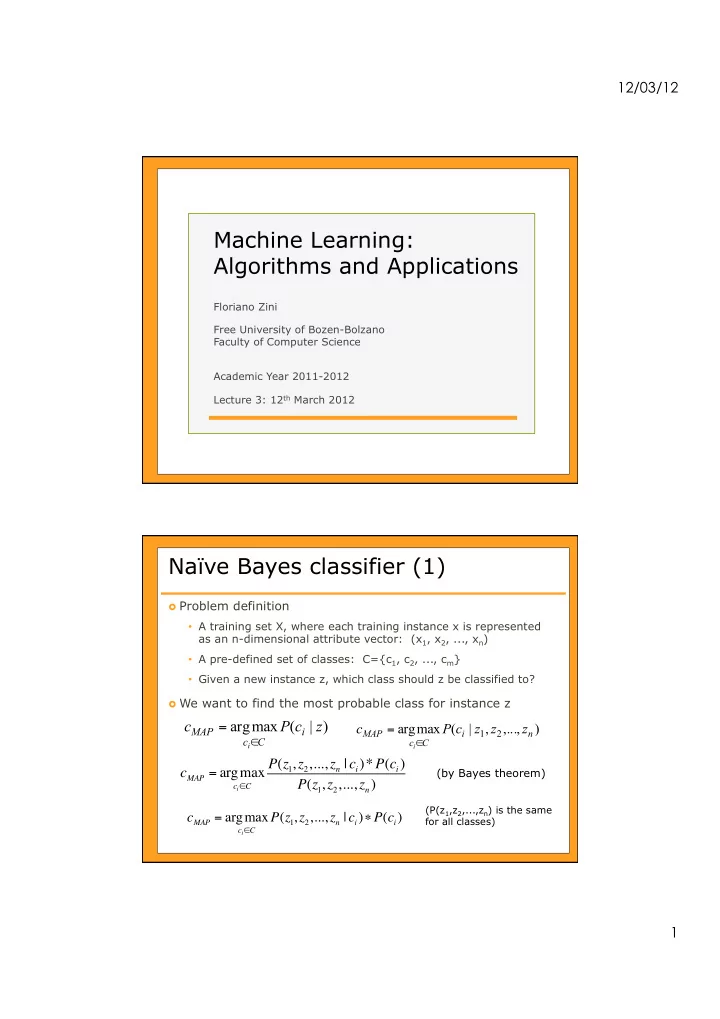
Naïve Bayes classifier (1)

 Problem definition

A training set X, where each training instance x is represented

as an n-dimensional attribute vector: (x1, x2, ..., xn)

A pre-defined set of classes: C={c1, c2, ..., cm}
Given a new instance z, which class should z be classified to?

 We want to find the most probable class for instance z

) | ( max arg z c P c

i C c MAP

i∈

=

) ,..., , | ( max arg

2 1 n i C c MAP

z z z c P c

i∈

=

cMAP = argmax

ci!C

P(z1, z2,..., zn | ci)*P(ci) P(z1, z2,..., zn)

(by Bayes theorem)

cMAP = argmax

ci!C

P(z1, z2,..., zn | ci)"P(ci)

(P(z1,z2,...,zn) is the same for all classes)

SLIDE 2

12/03/12 2

Naïve Bayes classifier (2)

Assumption in Naïve Bayes classifier. The attributes are conditionally independent given the classification

∏

=

n j i j i n

c z P c z z z P

1 2 1

) | ( ) | ,..., , ( Naïve Bayes classifier finds the most probable class for z

cNB = argmax

ci!C

P(ci)* P(zj | ci)

j=1 n

"

Naïve Bayes classifier - Algorithm

 The learning (training) phase (given a training set)

For each class ci∈C

Estimate the prior probability: P(ci)
For each attribute value zj, estimate the probability of that

attribute value given class ci: P(zj|ci)

 The classification phase

For each class ci∈C, compute the formula

P(ci)! P(zj | ci)

j=1 n

"

Select the most probable class c*

c* = argmax

ci!C

P(ci)" P(zj | ci)

j=1 n

#

SLIDE 3

12/03/12 3

Naïve Bayes classifier – Example (1)

Will a young student with medium income and fair credit rating buy a computer?

Rec. ID

Age Income Student Credit_Rating Buy_Computer 1 Young High No Fair No 2 Young High No Excellent No 3 Medium High No Fair Yes 4 Old Medium No Fair Yes 5 Old Low Yes Fair Yes 6 Old Low Yes Excellent No 7 Medium Low Yes Excellent Yes 8 Young Medium No Fair No 9 Young Low Yes Fair Yes 10 Old Medium Yes Fair Yes 11 Young Medium Yes Excellent Yes 12 Medium Medium No Excellent Yes 13 Medium High Yes Fair Yes 14 Old Medium No Excellent No

http://www.cs.sunysb.edu/~cse634/lecture_notes/07classification.pdf

Naïve Bayes classifier – Example (2)

 Representation of the problem

z = (Age=Young,Income=Medium,Student=Yes,Credit_Rating=Fair)
Two classes: c1 (buy a computer) and c2 (not buy a computer)

 Compute the prior probability for each class

P(c1) = 9/14
P(c2) = 5/14

 Compute the probability of each attribute value given each

class

P(Age=Young|c1) = 2/9;

P(Age=Young|c2) = 3/5

P(Income=Medium|c1) = 4/9;

P(Income=Medium|c2) = 2/5

P(Student=Yes|c1) = 6/9;

P(Student=Yes|c2) = 1/5

P(Credit_Rating=Fair|c1) = 6/9;

P(Credit_Rating=Fair|c2) = 2/5

SLIDE 4

12/03/12 4

Naïve Bayes classifier – Example (3)

 Compute the likelihood of instance z given each class

For class c1

For class c2

For class c1

P(c1)*P(z|c1) = (9/14)*(0.044) = 0.028

For class c2

P(c2)*P(z|c2) = (5/14)*(0.019) = 0.007

→ Conclusion: The person z (a young student with medium income and fair credit rating) will buy a computer!

Naïve Bayes classifier – Issues (1)

 What happens if no training instances associated with class ci have

attribute value xj?

 E.g., in the “buy computer” example, no young students bought computers

P(xj|ci)= n(cj,xj)/n(cj)=0 , and hence:

 Solution: use a Bayesian approach to estimate P(xj|ci)

n(ci): number of training instances associated with class ci
n(ci,xj): number of training instances associated with class ci that have attribute

value xj

p: a prior estimate for P(xj|ci)

→ Assume uniform priors: p=1/k, if attribute fj has k possible values

m: a weight given to prior

→ To augment the n(ci) actual observations by an additional m virtual samples distributed according to p

P(ci)! P(x j | ci)

j=1 n

"

= 0 m c n mp x c n c x P

i j i i j

+ + = ) ( ) , ( ) | (

SLIDE 5

12/03/12 5

Naïve Bayes classifier – Issues (2)

P(xj|ci)<1, for every attribute value xj and class ci
So, when the number of attribute values is very

large

) | ( lim

1

= ⎟ ⎟ ⎠ ⎞ ⎜ ⎜ ⎝ ⎛∏

= ∞ → n j i j n

c x P

n Solution: use a logarithmic function of probability

cNB = argmax

ci!C

log P(ci)" P(x j | ci)

j=1 n

#

$ % & & ' ( ) ) * + , ,

.

/ / ⎟ ⎟ ⎠ ⎞ ⎜ ⎜ ⎝ ⎛ + =

∑

= ∈ n j i j i C c NB

c x P c P c

i

1

) | ( log ) ( log max arg

Naïve Bayes classifier – Summary

 One of the most practical learning methods  Based on the Bayes theorem  Parameter estimation for Naïve Bayes models uses the maximum likelihood

estimation

 Computationally very fast

Training: only one pass over the training set
Classification: linear in the number of attributes

 Despite its conditional independence assumption, Naïve Bayes classifier

shows a good performance in several application domains

 When to use?

A moderate or large training set available
Instances are represented by a large number of attributes
Attributes that describe instances are conditionally independent given

classification

SLIDE 6

12/03/12 6

Linear regression Linear regression – Introduction

 Goal: to predict a real-valued output given an input instance  A simple-but-effective learning technique when the target

function is a linear function

 The learning problem is to learn (i.e., approximate) a real-valued

function f f: X → Y

X: The input domain (i.e., an n-dimensional vector space – Rn)
Y: The output domain (i.e., the real values domain – R)
f: The target function to be learned (i.e., a linear mapping function)

 Essentially, to learn the weights vector

w = (w0, w1, w2, …, wn)

∑

=

+ = + + + + =

n i i i n n

x w w x w x w x w w x f

1 2 2 1 1

... ) (

(wi,xi ∈R)

SLIDE 7

12/03/12 7

Linear regression – Example

What is the linear function f(x)?

f(x) x x f(x)

0.13

0.91

1.02

0.17

3.17 1.61

2.76
3.31

1.44 0.18 5.28 3.36

1.74
2.46

7.93 5.56 ... ...

E.g., f(x) = -1.02 + 0.83x

Linear regression – Training / test instances

 For each training instance x=(x1,x2,...,xn) ∈ X, where xi∈R

The desired (target) output value cx (∈R)
The actual output value

→ Here, wi are the system’s current estimates of the weights → The actual output value yx is desired to (approximately) be cx

 For a test instance z=(z1,z2,...,zn)

To predict the output value
By applying the learned target function f

∑

=

+ =

n i i i x

x w w y

1

SLIDE 8

12/03/12 8

Linear regression – Error function

 The learning algorithm requires to define an error

function

→ To measure the error made by the system in the training phase

 Definition of the training square error E

Error computed on each training example x:
Error computed on the entire training set X:

2 1 2

2 1 ) ( 2 1 ) ( ⎟ ⎟ ⎠ ⎞ ⎜ ⎜ ⎝ ⎛ − − = − =

∑

= n i i i x x x

x w w c y c x E

E = E(x)

x!X

"

= 1 2 (cx # yx)2 = 1 2

x!X

"

cx # w0 # wixi

i=1 n

"

$ % & ' ( )

x!X

"

2

Least-square linear regression

 Learning the target function f is equivalent to learning the

weights vector w that minimizes the training square error E

→ Why the name of the approach is “Least-Square Linear Regression”

 Training phase

Initialize the weights vector w (small random values)
Compute the training error E
Update the weights vector w according to the delta rule
Repeat until converging to a (locally) minimum error E

 Prediction phase

For a new instance z, the (predicted) output value is:

∑

=

+ =

n i i i z

w w z f

1

* * ) (

where w*=(w*0,w*1,..., w*n) is the learned weights vector

SLIDE 9

12/03/12 9

The delta rule

 To update the weights vector w in the direction that

decreases the training error E

η is the learning rate (i.e., a small positive constant)

→ To decide the degree to which the weights are changed at each training step

Instance-to-instance update: wi ← wi + η(cx-yx)xi
Batch update:

 Other names of the delta rule

LMS (least mean square) rule
Adaline rule
Widrow-Hoff rule

wi ! wi +! cx " yx

( )

x#X

$

xi

LSLR_batch(X, η)

for each attribute i wi ← an initial (small) random value while not CONVERGENCE for each attribute i delta_wi ← 0 for each training example x∈X compute the actual output value yx for each attribute i delta_wi ← delta_wi + η(cx-yx)xi for each attribute i wi ← wi + delta_wi end while return w

SLIDE 10

12/03/12 10

Batch vs. incremental update

 The previous algorithm follows a batch update approach  Batch update

At each training step (cycle), the weights are updated after all

the training instances are inputted to the system

First, the error is computed cumulatively on all the training

instances

Then, the weights are updated according to the overall

(cumulated) error  Incremental update

At each training step, the weights are updated immediately

after each training instance is inputted to the system

The individual error is computed for the training instance
The weights are updated immediately according to the individual

error

LSLR_incremental(X, η) for each attribute i wi ← an initial (small) random value while not CONVERGENCE for each training example x∈X compute the actual output value yx for each attribute i wi ← wi + η(cx-yx)xi end while return w

SLIDE 11

12/03/12 11

Training termination conditions

 In the LSLR_batch and LSLR_incremental learning

algorithms, the training process terminates when the conditions indicated by CONVERGENCE are met

 The (training) termination conditions are typically defined

based on some kind of system performance measure

Stop, if the error is less than a threshold value
Stop, if the error at a learning step is greater than that at the

previous step

Stop, if the difference between the errors at two consecutive steps is

less than a threshold value

Stop, if ...

Nearest neighbor learner

SLIDE 12

12/03/12 12

Nearest neighbor learner – Introduction (1)

 Some alternative names

Instance-based learning
Lazy learning
Memory-based learning

 Nearest neighbor learner

Given a set of training instances

─ Just store the training instances ─ Not construct a general, explicit description (model) of the

target function based on the training instances

Given a test instance (to be classified/predicted)

─ Examine the relationship between the test instance and the

training instances to assign a target function value

Nearest neighbor learner – Introduction (2)

 The input representation

Each instance x is represented as a vector in an n-

dimensional vector space X∈Rn

x = (x1,x2,…,xn), where xi (∈R) is a real number

 We consider two learning tasks

Nearest neighbor learner for classification

─ To learn a discrete-valued target function ─ The output is one of pre-defined nominal values (i.e., class

labels)

Nearest neighbor learner for prediction

─ To learn a continuous-valued target function ─ The output is a real number

SLIDE 13

12/03/12 13

Nearest neighbor learner – Example

 1 nearest neighbor

→ Assign z to c2

 3 nearest neighbors

→ Assign z to c1

 5 nearest neighbors

→ Assign z to c1

test instance z class c1 class c2

k-Nearest neighbor classifier – Algorithm

 For the classification task  Each training instance x is represented by

The description: x=(x1,x2,…,xn), where xi∈R
The class label: c (∈C, where C is a pre-defined set of class labels)

 Training phase

Just store the training instances set X = {x}

 Test phase. To classify a new instance z

For each training instance x∈X, compute distance between x and z
Compute the set NB(z) – the neighbourhood of z

→ The k instances in X nearest to z according to a distance function d

Classify z to the majority class of the instances in NB(z)

SLIDE 14

12/03/12 14

k-Nearest neighbor predictor – Algorithm

 For the regression task (i.e., to predict a real output value)  Each training instance x is represented by

The description: x=(x1,x2,…,xn), where xi∈R
The output value: yx∈R (i.e., a real number)

 Training phase

Just store the training examples set X

 Test phase. To predict the output value for new instance z

For each training instance x∈X, compute distance between x and z
Compute the set NB(z) – the neighbourhood of z

→ The k instances in X nearest to z according to a distance function d

Predict the output value of z:

∑ ∈

=

) (

1

z NB x x z

y k y

One vs. More than one neighbor

 Using only a single neighbor (i.e., the training

instance closest to the test instance) to determine the classification is subject to errors

E.g., noise (i.e. error) in the class label of a single training

instance

 Consider the k (>1) nearest training instances, and

return the majority class label of these k instances

 The value of k is typically odd to avoid ties

For example, k=3 or k=5

SLIDE 15

12/03/12 15

Distance function (1)

 The distance function d

Play a very important role in the nearest neighbor

learning approach

Typically defined before, and fixed through, the training

and test phases – i.e., not adjusted based on data

 Choice of the distance function d

Geometry distance functions, for continuous-valued input

space (xi∈R)

Hamming distance function, for binary-valued input space

(xi∈{0,1})

Distance function (2)

 Geometry distance functions

Manhattan distance
Euclidean distance
Minkowski (p-norm) distance
Chebyshev distance

∑

=

− =

n i i i

z x z x d

1

) , (

( )

∑

=

− =

n i i i

z x z x d

1 2

) , (

p n i p i i

z x z x d

/ 1 1

) , ( ⎟ ⎠ ⎞ ⎜ ⎝ ⎛ − = ∑

= i i i

z x − = max

p n i p i i p

z x z x d

/ 1 1

lim ) , ( ⎟ ⎠ ⎞ ⎜ ⎝ ⎛ − =

∑

= ∞ →

SLIDE 16

12/03/12 16

Distance function (3)

 Hamming distance

function

For binary-valued input

space

E.g., x=(0,1,0,1,1)

∑

=

n i i i z

x Difference z x d

1

) , ( ) , ( ⎩ ⎨ ⎧ = ≠ = ) ( , ) ( , 1 ) , ( b a if b a if b a Difference

Attribute value normalization

 The Euclidean distance function  Assume that an instance is represented by 3 attributes: Age,

Income (per month), and Height (in meters)

x = (Age=20, Income=12000, Height=1.68)
z = (Age=40, Income=1300, Height=1.75)

 The distance between x and z

d(x,z) = [(20-40)2 + (12000-1300)2 + (1.68-1.75)2]1/2
The distance is dominated by the local distance (difference) on the

Income attribute → Because the Income attribute has a large range of values

 To normalize the values of all the attributes to the same range

Usually the value range [0,1] is used
E.g., for every attribute i: xi = xi/max_value_of_attribute_i

( )

∑

=

− =

n i i i

z x z x d

1 2

) , (

SLIDE 17

12/03/12 17

Attribute importance weight

 The Euclidean distance function

All the attributes are considered equally important in the distance

computation

 Different attributes may have different degrees of influence on

the distance metric

 To incorporate attribute importance weights in the distance

function

wi is the importance weight of attribute i:

 How to achieve the attribute importance weights?

By the domain-specific knowledge (e.g., indicated by experts in

the problem domain)

By an optimization process (e.g., using a separate validation set

to learn an optimal set of attribute weights)

( )

∑

=

− =

n i i i

z x z x d

1 2

) , (

( )

∑

=

− =

n i i i i

z x w z x d

1 2

) , (

Distance-weighted NN learner (1)

 Consider NB(z) – the set of the k

training instances nearest to the test instance z

Each (nearest) instance has a

different distance to z

Should these (nearest) instances

influence equally to the classification/prediction of z? → No!

 To weight the contribution of each

f the k neighbors according to

their distance to z

Larger weight for nearer neighbor!

test instance z

SLIDE 18

12/03/12 18

Distance-weighted NN learner (2)

 Let’s denote by v a distance-based weighting

function

Given a distance d(x,z) – the distance of x to z
v(x,z) is inversely proportional to d(x,z)

 For the classification task:  For the prediction task:  Select a distance-based weighting function

c(z) = argmax

cj !C

v(x, z)"!(cj,c(x))

x!NB(z)

#

!(a,b) = 1,if (a = b) 0,if (a ! b) " # $ % $ f (z) = v(x, z)! f (x)

x"NB(z)

#

v(x, z)

x"NB(z)

#

) , ( 1 ) , ( z x d z x v + = α

2

)] , ( [ 1 ) , ( z x d z x v + = α

2 2

) , (

σ z x d

e z x v

−

=

Lazy learning vs. Eager learning

 Lazy learning. The target function estimation (i.e., generalization)

is postponed until the test instance is introduced

E.g., Nearest neighbor learner, Locally weighted regression
Estimate (i.e., approximate) the target function locally and differently for each test

instance – i.e., performed at the classification/prediction time

Compute many local approximations of the target function
Typically take longer time to answer queries, and require more memory space

 Eager learning. The target function estimation is completed before

any test instance is introduced

E.g., Linear regression, Support vector machines, Neural networks, etc.
Estimate (i.e., approximate) the target function globally for the entire instance

space – i.e., performed at the training time

Compute a single (global) approximation of the target function

SLIDE 19

12/03/12 19

Nearest neighbor learner – When?

 Instances are represented as vectors in Rn  The dimensionality of the input space is not large  A large set of training instances is available

 Advantages

No training is needed (i.e., just store the training instances)
Scale well with a large number of classes

→ Not need to learn n classifiers for n classes

k-NN (k >>1) learner is robust to noisy data

→ Classification/prediction is performed considering k nearest neighbors  Disadvantages

Distance function must be carefully chosen
Computational cost (in time and memory) at the classification/prediction time
May be misled by irrelevant attributes