Computational Anatomy: Simple Statistics on Interesting Spaces - - PDF document

1

10/21/2005 Sarang Joshi MICCAI 2005

Computational Anatomy: Simple Statistics on Interesting Spaces

Sarang Joshi, Brad Davis, Peter Lorenzen and Guido Gerig

Departments of Radiation Oncology, Biomedical Engineering and Computer Science University of North Carolina at Chapel Hill

10/21/2005 Sarang Joshi MICCAI 2005

Computation Anatomy

• Precise Computational study of Anatomical Variability.
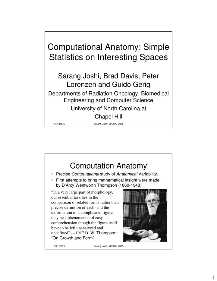
• First attempts to bring mathematical insight were made

by D’Arcy Wentworth Thompson (1860-1948) “In a very large part of morphology,

• ur essential task lies in the

comparison of related forms rather than precise definition of each; and the deformation of a complicated figure may be a phenomenon of easy comprehension though the figure itself have to be left unanalyzed and undefined” ---1917 D. W. Thompson: “On Growth and Form”

2

10/21/2005 Sarang Joshi MICCAI 2005

Image Understanding Via Computational Anatomy

• Deformable Image Registration. Map a family of

images to a single Template Image

10/21/2005 Sarang Joshi MICCAI 2005

Motivation:A Natural Question

• Given a collection of Anatomical Images

what is the Image of the “Average Anatomy”

3

10/21/2005 Sarang Joshi MICCAI 2005

Motivation: A Natural Question

What is the Average? Consider two simple images of circles:

10/21/2005 Sarang Joshi MICCAI 2005

Motivation: A Natural Question

What is the Average? Consider two simple images of circles:

4

10/21/2005 Sarang Joshi MICCAI 2005

Motivation: A Natural Question

What is the Average?

10/21/2005 Sarang Joshi MICCAI 2005

Motivation: A Natural Question

Average considering “Geometric Structure”

A circle with “average radius”

5

10/21/2005 Sarang Joshi MICCAI 2005

Motivation: A Natural Question

Simple average:

10/21/2005 Sarang Joshi MICCAI 2005

Motivation: A Natural Question

Average considering “Geometric Structure”

6

10/21/2005 Sarang Joshi MICCAI 2005

Mathematical Foundations Computational Anatomy

• Homogeneous Anatomy characterized by
• :The underlying coordinate system with a collection of 0,1,2 and 3

dimensional compact manifolds of 0-Dimensional –Landmark points 1-Dimensional –Lines 2-Dimensional –Surfaces 3-Dimensional –Sub-Volumes

• A set of transformation of accommodating

biological variability.

• I Set of anatomical Imagery (CT, MRI, PET, US etc…)
• P: A probability measure on the set of transformation.

10/21/2005 Sarang Joshi MICCAI 2005

Interesting Spaces

• Image intensities I well represented by

elements of flat spaces:

– L2 :Square integrable functions.

• Structure in Images represented by

transformation groups:

– For circles simple multiplicative group of positive real’s (R+) – Scale and Orientation: Finite dimensional Lie Groups such as Rotations, Similarity and Affine Transforms. – High dimensional anatomical structural variation: Infinite dimensional Group of Diffeomorphisms

7

10/21/2005 Sarang Joshi MICCAI 2005

Space of Images and Anatomical Structure

• Images as function of a underlying coordinate

space

• Image intensities
• Space of structural transformations:

diffeomorphisms of the underlying coordinate space

• Space of Images and Transformations a semi-

direct product of the two spaces. ) (

2 Ω

L ) (Ω Diff Ω Ω

) ( ) (

2

Ω ⊗ Ω Diff L

10/21/2005 Sarang Joshi MICCAI 2005

Mathematical Foundations of Computational Anatomy

• transformations constructed from the group of

diffeomorphisms of the underlying coordinate system

– Diffeomorphisms: one-to-one onto (invertible) and differential

• transformations. Preserve topology.
• Anatomical variability understood via transformations

– Traditional approach: Given a family of images construct “registration” transformations that map all the images to a single template image or the Atlas.

• How can we define an “Average anatomy” in this

framework: The Atlas estimation problem!!

8

10/21/2005 Sarang Joshi MICCAI 2005

Large deformation diffeomorphisms

• Space of all Diffeomorphisms forms

a group under composition:

• Space of diffeomorphisms not a vector

space.

) (Ω Diff

) ( : ) ( ,

2 1 2 1

Ω ∈ = Ω ∈ ∀ Diff h h h Diff h h

• )

( : ) ( ,

2 1 2 1

Ω ∉ + = Ω ∈ ∀ Diff h h h Diff h h

10/21/2005 Sarang Joshi MICCAI 2005

Large deformation diffeomorphisms.

• infinite dimensional “Lei Group”

(Almost).

• Tangent space: The space of smooth velocity

fields.

• Construct deformations by integrating flows of

velocity fields.

) (Ω Diff

9

10/21/2005 Sarang Joshi MICCAI 2005

Large deformation diffeomorphisms.

• Proof: Existence and Uniqueness
• f solutions of ODE’s.
• One-to-one: Uniqueness
• Differentiability: Smooth dependence
• n initial condition.

10/21/2005 Sarang Joshi MICCAI 2005

Relationship to Fluid Deformations

• Newtonian fluid flows generate

diffeomorphisms: John P. Heller "An Unmixing

Demonstration," American Journal of Physics, 28, 348- 353 (1960).

10

10/21/2005 Sarang Joshi MICCAI 2005

Simple Statistics on Interesting Spaces: ‘Average Anatomy’

• Use the notion of Fréchet mean to define

the “Average Anatomical” image.

• The “Average Anatomical” image: The

image that minimizes the mean squared metric on the semi-direct product space

) ( ) (

2

Ω ⊗ Ω Diff L

10/21/2005 Sarang Joshi MICCAI 2005

Metric on the Group of Diffeomorphisms: LDMM

• Induce a metric via a Sobolev norm on the velocity fields.

Distance defined as the length of Geodesics under this norm.

• Distance between e, the identity and any diffeomorphism

ϕ is defined via the geodesic equation:

• Left invariant distance between any two is defined as:

11

10/21/2005 Sarang Joshi MICCAI 2005

Simple Statistics on Interesting Spaces: ‘Averaging Anatomies’

• The average anatomical image is the Image that

requires “Least Energy to deform and match to all the Images in a population”:

• Not as intractable as it looks!!
• Efficient alternating algorithm:

10/21/2005 Sarang Joshi MICCAI 2005

Simple Statistics on Interesting Spaces: ‘Averaging Images’

• If the transformations are fixed than the average

image is simply the average of the deformed images!!

• Alternate until convergence between estimating

the average and the transformations.

12

10/21/2005 Sarang Joshi MICCAI 2005

Results: Sample of 16 Bull’s eye Images

10/21/2005 Sarang Joshi MICCAI 2005

Averaging of 16 Bull’s eye images

13

10/21/2005 Sarang Joshi MICCAI 2005

Averaging of 16 Bull’s eye images

Voxel Averaging LDMM Averaging

Numerical average of the radii of the individual circles forming the bulls eye sample.

10/21/2005 Sarang Joshi MICCAI 2005

Applications: Early Brain Development Assessed by structural MRI

• Longitudinal study of Brain

Growth from 2 Years to 4 Years.

• Quantify details Structural

differences.

14

10/21/2005 Sarang Joshi MICCAI 2005

Applications: Early Brain Development Assessed by structural MRI

10/21/2005 Sarang Joshi MICCAI 2005

Applications: Early Brain Development Assessed by structural MRI

15

10/21/2005 Sarang Joshi MICCAI 2005

Applications: Early Brain Development Assessed by structural MRI

10/21/2005 Sarang Joshi MICCAI 2005

Applications: Early Brain Development Assessed by structural MRI

• Deformation between 2 Year

Average and 4 Year Average.

16

10/21/2005 Sarang Joshi MICCAI 2005

Applications: Early Brain Development Assessed by structural MRI

• Full volumetric analysis of Brain Growth.
• Use Log-Jacobian to study local volumetric

changes.

10/21/2005 Sarang Joshi MICCAI 2005

How many images do we need to build a stable population?

For more details see: P. Lorenzen, B. Davis, and S. Joshi, "Unbiased Atlas Formation via Large Deformations Metric Mapping", in MICCAI 2005 , Pages 411- 418.

17

10/21/2005 Sarang Joshi MICCAI 2005

References

• Computational Anatomy

–

• U. Grenander and M. I. Miller, "Computational Anatomy: An Emerging Discipline," Quarterly
• f Applied Mathematics, vol. 56, no. , pp. 617-694, 1998.
• Diffeomorphic image registration

–

• G. E. Christensen, R. D. Rabbitt, and M. I. Miller, "Deformable Templates Using Large

Deformation Kinematics," IEEE Transactions on Image Processing, vol. 5, no. 10, pp. 1435- 1447, Oct. 1996. –

• G. E. Christensen, S. C. Joshi, and M. I. Miller, "Volumetric Transformation of Brain

Anatomy," IEEE Transactions on Medical Imaging, vol. 16, no. 6, pp. 864-877, Dec. 1997. –

• S. Joshi and M. I. Miller, "Landmark Matching Via Large Deformation Diffeomorphisms,"

IEEE Transactions on Image Processing, vol. 9, no. 8, pp. 1357-1370, Aug. 2000. – M.I. Miller and L. Younes, "Group Actions, Homeomorphisms, and Matching: A General Framework", International Journal of Computer Vision, Volume 41, No 1/2, pages 61-84, 2001

• Atlas Construction

– Sarang Joshi, Brad Davis, Matthieu Jomier, and Guido Gerig, "Unbiased Diffeomorphic Atlas Construction for Computational Anatomy," NeuroImage; Supplement issue on Mathematics in Brain Imaging, vol. 23, no. Supplement1, pp. S151-S160, Elsevier, Inc, 2004. –

• P. Lorenzen, B. Davis, and S. Joshi, "Unbiased Atlas Formation via Large Deformations

Metric Mapping", in MICCAI 2005 , Pages 411-418. 10/21/2005 Sarang Joshi MICCAI 2005

Hypothesis Testing with Nonlinear Shape Models

Timothy B. Terriberry, Sarang C. Joshi, and Guido Gerig

• Dept. of Computer Science,
• Univ. of North Carolina at Chapel Hill

18

10/21/2005 Sarang Joshi MICCAI 2005

Hypothesis Testing

• The goal: To determine if two different

populations of objects have significant shape differences

10/21/2005 Sarang Joshi MICCAI 2005

Hypothesis Testing

• The challenges:

–High dimension, low sample size –Shape parameters live in non- Euclidean spaces –Different variables are not commensurate –Neighboring sites are correlated

19

10/21/2005 Sarang Joshi MICCAI 2005

Shape Model: M-reps

• 8 dimensions per

medial atom

– x (3), r (1), n0 (2), n1 (2)

• Riemannian

symmetric space

– R3×R+×S2×S2 (Fletcher et al. 2003) – Nonlinear, except R3

10/21/2005 Sarang Joshi MICCAI 2005

Metric Space

• Each parameter has a metric invariant to geometric

transformations – R3 - Euclidean metric (invariant to translation) – R+ - |log(r1) - log(r2)| (invariant to scale) – S2 - Distance on sphere (invariant to rotation)

• Can define the Fréchet mean of populations via the metric.
• Cannot do statistical testing on the tangent space as the two

populations have different means and hence different tangent spaces – No way to intrinsically transform covariance structure from one tangent space to another especially if the manifold is not parallizable.

∑

∈

=

i i M x

x x d

2

) , ( min arg ˆ µ

20

10/21/2005 Sarang Joshi MICCAI 2005

Our Approach

• Generalize permutation tests to capture

desirable properties of Hotelling's test

– Use a true multivariate permutation test framework (Pesarin 2001)

• Perform partial tests on individual features
• Combine the test results into a single score

– Trivial example: Bonferroni correction

• min p-value multiplied by number of tests
• Too pessimistic for high-dimension data

10/21/2005 Sarang Joshi MICCAI 2005

Our Approach

• Marginal permutation tests on

individual features generate uniformly distributed and parameterization invariant p-values

• Using a c.d.f., map the uniform

distribution to a standard distribution, and perform tests there

• Gives an unbiased global test for

equality of population distributions

21

10/21/2005 Sarang Joshi MICCAI 2005

Our Approach In Pictures

10/21/2005 Sarang Joshi MICCAI 2005

Example

• Two data sets

– Size n1 = n2 = 10

• M=2 dimensional

feature vectors – Position, Scale

• Drawn from multivariate normal distributions

(common covariance) – Second parameter exponentiated – Then both parameters scaled by 10

22

10/21/2005 Sarang Joshi MICCAI 2005

Step 1: Partial Tests

• Choose N random

assignments to group 1 or 2

• For each feature j

and permutation k

– Compute a test statistic , e.g. – Also compute , the statistics for the

• bserved data

k j

T ) ˆ , ˆ (

, 2 , 1 k j k j

d µ µ

• j

T

10/21/2005 Sarang Joshi MICCAI 2005

Step 2: Partial Test p-values

• For each feature j

and permutation k

– Compute a p-value using that feature's cumulative distribution:

• The marginal distributions are uniform,

and invariant to scale

( ) ( )

k j l j N = l k j

T , T H N = T p

∑

1

1

( )

⎪ ⎩ ⎪ ⎨ ⎧ ≥

l j k j l j k j k j l j

T < T T T = T , T H 0, 1,

23

10/21/2005 Sarang Joshi MICCAI 2005

Step 3: Combined Test

• If the partial tests are

– Significant for large values – Consistent – Marginally unbiased (unbiased regardless of whether

• r not other tests are true)
• And we choose a combining function T'(p(T k)) such

that it is – Monotonically non-increasing in each p-value – Obtains its supremum T* when any p-value is 0 – Has finite critical values strictly smaller than T*

10/21/2005 Sarang Joshi MICCAI 2005

Step 3: Combined Test

• Theorem: Then T'(p(T k)) is an unbiased

global test for equality of distributions (Pesarin 2001)

• What function should we use?
• One asymptotically equivalent to Hotelling's

T2 test (in linear case)

– Uniformly most powerful, and affine invariant

24

10/21/2005 Sarang Joshi MICCAI 2005

Step 3: Combined Test (2- sided)

• With signed distances, is significant for

large and small values

• Map p-values for each feature to a standard

normal distribution Gaussian c.d.f.

• Compute samp. covariance

– Full rank even for small samples: N is large

• Then

( )

k U T k k

U Σ U = T'

1 −

k j

T

), 2 1 ) ( (

1

N T P U

k j k j

− Φ =

−

: Φ

U U N

T U

1 = Σ

10/21/2005 Sarang Joshi MICCAI 2005

Acceptance Region

• Map critical

region via c.d.f. to

• riginal

space

• Contains

both axes (p- value = 0)

25

10/21/2005 Sarang Joshi MICCAI 2005

Application: Twin Ventricles

• MRI data of lateral ventricles from twin

pairs

– MZ - Healthy monozygotic: 9 pairs – DS - Monozygotic and discordant for schizophrenia: 9 pairs – DZ - Healthy dizygotic: 10 pairs – NR - Healthy non-related pairs: 10 pairs drawn from other healthy subjects

10/21/2005 Sarang Joshi MICCAI 2005

Application: Twin Ventricles

• Existing data set (provided by Martin

Styner) includes:

– Binary segmentations – PDM models of surface – M-rep models (3 × 13 grid, 98% volume overlap)

• All shapes volume normalized
• Aligned via m-rep extension of Procrustes

(Fletcher et al. 2004)

26

10/21/2005 Sarang Joshi MICCAI 2005

Application: Twin Ventricles

• Test: Is shape variability between pairs related

to genes? Disease?

• Test statistics for pairs (x1,y1) in group 1 and

(x2,y2) in group 2

• 6 features per atom (x (3), r (1),n0 (1), n1(1)),

39 atoms: M = 234 tests

• N = 50,000 permutations

( ) ( ) ( )

j i, j i, n = i j i, j i, n = i j

y , x d n y , x d n = y x y x T

1, 1, 1 1 1 2, 2, 2 1 2 2 2, 1, 1,

1 1

∑ ∑

−

10/21/2005 Sarang Joshi MICCAI 2005

Global Results

• Comparison of our results with an

earlier study on the PDMs (Styner et

• al. 2002)

– Tests significant at 0.05 level in bold

27

10/21/2005 Sarang Joshi MICCAI 2005

Local Tests

• Local tests (M = 6 partial tests per

atom, correction for multiple tests applied across atoms)

10/21/2005 Sarang Joshi MICCAI 2005

Conclusion

• Developed multivariate permutation

test approach for hypothesis testing

• Well-defined in HDLSS case
• Requires only a metric space
• Combines features of differing scale
• Multivariate approach accounts for

correlation, even without explicit correlation coefficients

28

10/21/2005 Sarang Joshi MICCAI 2005

References

• T Terriberry, S Joshi, and G Gerig,

"Hypothesis Testing with Nonlinear Shape Models," in Information Processing in Medical Imaging (IPMI), (G Christensen and M Sonka, eds.), (New York), pp. 15- 26, July 2005.

• Pesarin F (2001) Multivariate permutation

tests with applications in biostatistics. Wiley, Chichester, United Kingdom.