
SLIDE 1
Using Taylor Models in TTE 1
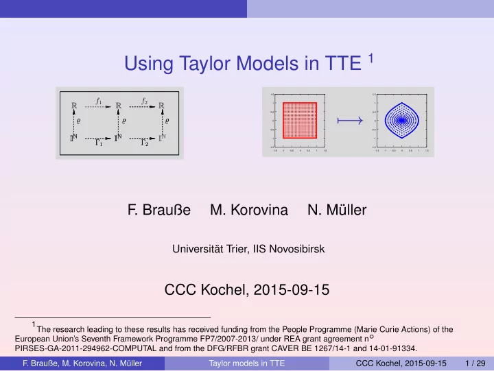
R f1 f2 R R ̺ ̺ ̺ Γ1 Γ2 ̺ ̺ ̺ Γ1 Γ2 IN IN IN IN IN
- 1.5
- 1
- 0.5
- 1.5
- 1
- 0.5
− →
- 1.5
- 1
- 0.5
- 1.5
- 1
- 0.5
F . Brauße
- M. Korovina
- N. Müller
Universität Trier, IIS Novosibirsk
CCC Kochel, 2015-09-15
1The research leading to these results has received funding from the People Programme (Marie Curie Actions) of the European Union’s Seventh Framework Programme FP7/2007-2013/ under REA grant agreement n◦ PIRSES-GA-2011-294962-COMPUTAL and from the DFG/RFBR grant CAVER BE 1267/14-1 and 14-01-91334.
- F. Brauße, M. Korovina, N. Müller
Taylor models in TTE CCC Kochel, 2015-09-15 1 / 29