Commutativity in Double Interchange Semigroups Murray Bremner Joint - PowerPoint PPT Presentation

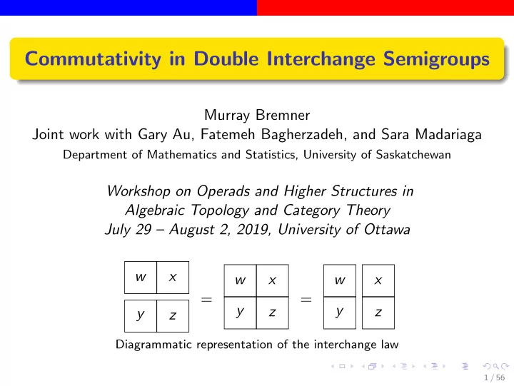
Commutativity in Double Interchange Semigroups Murray Bremner Joint work with Gary Au, Fatemeh Bagherzadeh, and Sara Madariaga Department of Mathematics and Statistics, University of Saskatchewan Workshop on Operads and Higher Structures in Algebraic Topology and Category Theory July 29 – August 2, 2019, University of Ottawa w x w x w x = = y y z z y z Diagrammatic representation of the interchange law 1 / 56

A very gentle introduction to higher-dimensional algebra 2 / 56

Horizontal and vertical multiplications Suppose that x and y are two indeterminates. When we compose x and y we usually write the result as xy . This composition may not be commutative: xy � = yx in general. We write the products xy and yx horizontally — but why? Why don’t we write the products vertically, y or x y ? x Paper (or blackboards, or computer screens, or . . . ) are 2-dimensional. Why don’t we use the third dimension (orthogonal to the screen)? We could write x in front of y , or y in front of x , using 3 dimensions. Is this just silly, or could it possibly have some important applications? Multiplying in different directions leads to higher-dimensional algebra . 3 / 56

From Ronald Brown’s survey paper Out of Line 4 / 56

A crossword puzzle: is this higher-dimensional algebra? 5 / 56

The interchange law for two operations y z Consider the 2 × 2 square product of four variables . w x There are two different ways to write this using ◦ and • : ( w ◦ x ) • ( y ◦ z ) or ( w • y ) ◦ ( x • z ) . Note the transpositions of x and y and of the operations ◦ and • . y z We assume these two ways of writing always give the same result. w x This assumption is called the interchange law : for all w , x , y , z we have ( w ◦ x ) • ( y ◦ z ) = ( w • y ) ◦ ( x • z ) . This relation between the two operations can be expressed as w x w x w x = = y y z z y z 6 / 56

The surprising Eckmann-Hilton argument (1) Assume that ◦ and • satisfy the interchange law: ( w ◦ x ) • ( y ◦ z ) = ( w • y ) ◦ ( x • z ) . Assume that ◦ and • have identity elements 1 ◦ and 1 • respectively. In the interchange law, take w = z = 1 ◦ and x = y = 1 • : ( ∗ ) (1 ◦ ◦ 1 • ) • (1 • ◦ 1 ◦ ) = (1 ◦ • 1 • ) ◦ (1 • • 1 ◦ ) . By definition of identity elements, 1 ◦ ◦ 1 • = 1 • ◦ 1 ◦ = 1 • , 1 ◦ • 1 • = 1 • • 1 ◦ = 1 ◦ . Using these to simplify equation ( ∗ ) gives 1 • • 1 • = 1 ◦ ◦ 1 ◦ . By definition of identity elements, this implies that 1 ◦ = 1 • . The two identity elements are equal. 7 / 56

The surprising Eckmann-Hilton argument (2) Write 1 for the common identity element: 1 = 1 ◦ = 1 • . In the interchange law, take w = z = 1: (1 ◦ x ) • ( y ◦ 1) = (1 • y ) ◦ ( x • 1) . By definition of identity element, this implies that x • y = y ◦ x . The black operation is the opposite of the white operation. Using this to simplify the interchange law gives ( y ◦ z ) ◦ ( w ◦ x ) = ( y ◦ w ) ◦ ( z ◦ x ) . Taking x = y = 1 in the last equation gives (1 ◦ z ) ◦ ( w ◦ 1) = (1 ◦ w ) ◦ ( z ◦ 1) . By definition of identity element, this implies that z ◦ w = w ◦ z . The white operation is commutative. 8 / 56

The surprising Eckmann-Hilton argument (3) But if x • y = y ◦ x , and y ◦ x = x ◦ y , then x • y = x ◦ y . The two operations are equal. (There is really only one operation.) Hence the interchange law can be simplified to ( w ◦ x ) ◦ ( y ◦ z ) = ( w ◦ y ) ◦ ( x ◦ z ) . Taking x = 1 gives ( w ◦ 1) ◦ ( y ◦ z ) = ( w ◦ y ) ◦ (1 ◦ z ) . By definition of identity element, this implies w ◦ ( y ◦ z ) = ( w ◦ y ) ◦ z . The operation is associative. We have proved the (in)famous Eckmann-Hilton Theorem . 9 / 56

The Eckmann-Hilton Theorem Theorem (Eckmann-Hilton) Let S be a set with two binary operations S × S → S denoted ◦ and • . Suppose that these two operations satisfy the interchange law. Suppose also that these two operations have identity elements 1 ◦ and 1 • . Then the two identity elements are equal, the two operations are equal, and the single remaining operation is both commutative and associative. Beno Eckmann, Peter Hilton : Group-like structures in general categories, I: Multiplications and comultiplications. Mathematische Annalen 145 (1961/62) 227–255. • Theorem 3.33 (page 236) • The definition of H -structure (page 241) • Theorem 4.17 (page 244) 10 / 56

A brief digression on homotopy groups The homotopy groups for n ≥ 1 of a topological space are defined in terms of continuous maps of the n -sphere into the space. The first homotopy group (the fundamental group) is defined in terms of loops in the space, and is usually noncommutative. Corollary (of the Eckmann-Hilton Theorem) For n ≥ 2 the higher homotopy groups are always commutative. Ronald Brown : groupoids.org.uk (slightly edited quotation) “The nonabelian fundamental group gave more information than the first homology group. Topologists were seeking higher dimensional versions of the fundamental group. ˇ Cech submitted to the 1932 ICM a paper on higher homotopy groups. These were quickly proved to be abelian in dimensions > 1, and Cech was asked (by Alexandrov and Hopf) to withdraw his paper. Only a short paragraph appeared in the Proceedings.” 11 / 56

Familiar examples of the interchange law (1) Example (multiplication and division) Suppose that the underlying set is the nonzero real numbers R \ { 0 } . Let the operations ◦ and • be multiplication and division, respectively. Then the interchange law states that ( w · x ) / ( y · z ) = ( w / y ) · ( x / z ) , which is simply the familiar rule for multiplying fractions: w · x y · z = w y · x z . (Why does the Eckmann-Hilton Theorem not imply that multiplication and division are the same commutative associative operation?) 12 / 56

Familiar examples of the interchange law (2) Example (composition of functions on Cartesian products) Suppose that ◦ denotes the operation of forming an ordered pair: f 1 ◦ f 2 = ( f 1 , f 2 ). Suppose that • denotes the operation of function composition: ( f • g )( − ) = f ( g ( − )). What does the interchange law state in this setting? ( f 1 ◦ f 2 ) • ( g 1 ◦ g 2 ) = ( f 1 • g 1 ) ◦ ( f 2 • g 2 ) ⇐ ⇒ � � � � � ( f 1 , f 2 ) • ( g 1 , g 2 ) ( − , − ) = ( f 1 • g 1 )( − ) , f 2 • g 2 )( − ) . The interchange law shows how to define composition of Cartesian products of functions on Cartesian products of sets. 13 / 56

Familiar examples of the interchange law (3) Example (endomorphism PROP of a set) Let X be a nonempty set, and let X n be its n -th Cartesian power ( n ≥ 1). Let Map ( m , n ) be the set of all functions f : X m → X n for m , n ≥ 1. Let Map ( X ) be the disjoint union of the sets Map ( m , n ): � Map ( X ) = Map ( m , n ) m , n ≥ 1 On Map ( X ) there are two natural binary operations: For f : X p → X q and g : X r → X s we define The horizontal product ◦ : the operation ◦ : Map ( p , q ) × Map ( r , s ) − → Map ( p + r , q + s ) as follows: ( f , g ) f ◦ g : X p + r = X p × X r → X q × X s = X q + s . − − − − − − This operation is defined for all p , q , r , s ≥ 1. 14 / 56

Example (continued) For f : X q → X r and g : X p → X q we define The vertical product • : the operation • : Map ( q , r ) × Map ( p , q ) − → Map ( p , r ) as follows: f • g f • g : X p → X r . − − − − − − This operation is defined on Map ( q 1 , r ) × Map ( p , q 2 ) only if q 1 = q 2 . These two operations satisfy the interchange law: ( f ◦ g ) • ( h ◦ k ) = ( f • h ) ◦ ( g • k ) . To verify this: compare the following maps, check the results are equal: ( h , k ) ( f , g ) ( f ◦ g ) • ( h ◦ k ): X p × X q → X r × X s → X t × X u , − − − − − − − − − − − − ( f • h ) ◦ ( g • k ): X p × X q ( f • h , g • k ) → X t × X u . − − − − − − − − − − 15 / 56

Familiar examples of the interchange law (4) Definition A double category D is a pair of categories ( D 0 , D 1 ) with functors e : D 0 → D 1 (identity map), s , t : D 1 → D 0 (source and target objects). In D 0 we denote objects by capital Latin letters A , . . . (the 0-cells of D ) and morphisms by arrows labelled by lower-case italic letters u , . . . (the vertical 1-cells of D ). In D 1 the objects are arrows labelled by lower-case italic letters h , . . . (the horizontal 1-cells of D ), and the morphisms are arrows labelled by lower-case Greek letters α , β , . . . (the 2-cells of D ). If A is an object in D 0 then e ( A ) is the (horizontal) identity arrow on A . (By Eckmann-Hilton, identity arrows may exist in only one direction.) The functors s , t are source and target : if h is a horizontal arrow in D 1 then s ( h ) and t ( h ) are its domain and codomain, objects in D 0 . These functors satisfy the equation s ( e ( A )) = t ( e ( A )) = A for every A . 16 / 56