
SLIDE 1
Comments on Choice of ARMA model
- Keep it simple! Use small p and q.
- Some systems have autoregressive-like structure.
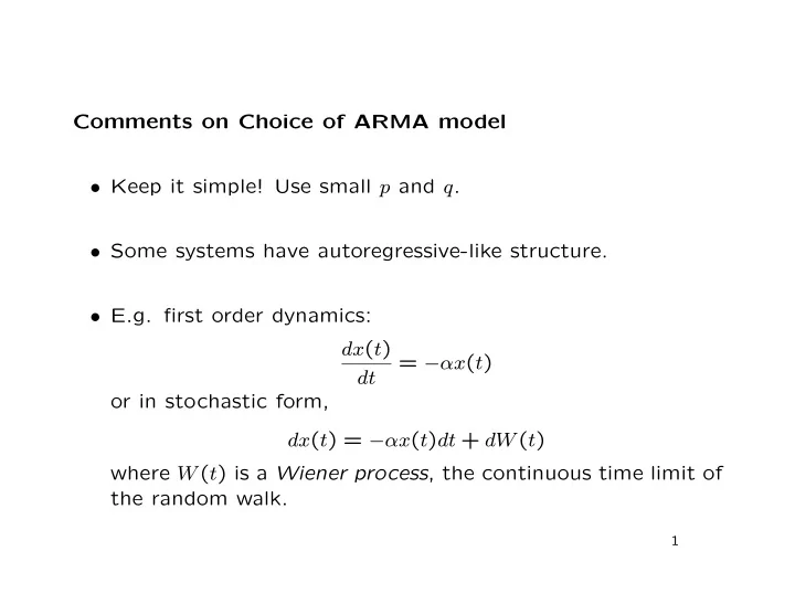
- E.g. first order dynamics:
dx(t) dt = −αx(t)
- r in stochastic form,