
SLIDE 1
Cold planar horizons are floppy
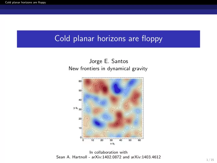
Cold planar horizons are floppy
Jorge E. Santos
New frontiers in dynamical gravity
In collaboration with Sean A. Hartnoll - arXiv:1402.0872 and arXiv:1403.4612
1 / 15
Cold planar horizons are floppy Jorge E. Santos New frontiers in - - PowerPoint PPT Presentation
Cold planar horizons are floppy Cold planar horizons are floppy Jorge E. Santos New frontiers in dynamical gravity In collaboration with Sean A. Hartnoll - arXiv:1402.0872 and arXiv:1403.4612 1 / 15 Cold planar horizons are floppy Motivation
Cold planar horizons are floppy
In collaboration with Sean A. Hartnoll - arXiv:1402.0872 and arXiv:1403.4612
1 / 15
Cold planar horizons are floppy
2 / 15
Cold planar horizons are floppy
2 / 15
Cold planar horizons are floppy
2 / 15
Cold planar horizons are floppy
2 / 15
Cold planar horizons are floppy
2 / 15
Cold planar horizons are floppy
2 / 15
Cold planar horizons are floppy
2 / 15
Cold planar horizons are floppy
2 / 15
Cold planar horizons are floppy
2 / 15
Cold planar horizons are floppy Outline
3 / 15
Cold planar horizons are floppy The Einstein-Maxwell system
4 / 15
Cold planar horizons are floppy The Einstein-Maxwell system
4 / 15
Cold planar horizons are floppy The Einstein-Maxwell system
4 / 15
Cold planar horizons are floppy The Einstein-Maxwell system
∂ = −dt2 + dx2 + dw2
4 / 15
Cold planar horizons are floppy The Einstein-Maxwell system
∂ = −dt2 + dx2 + dw2
4 / 15
Cold planar horizons are floppy The Einstein-Maxwell system
∂ = −dt2 + dx2 + dw2
4 / 15
Cold planar horizons are floppy The Einstein-Maxwell system
∂ = −dt2 + dx2 + dw2
4 / 15
Cold planar horizons are floppy Breakdown of Perturbation theory
5 / 15
Cold planar horizons are floppy Breakdown of Perturbation theory
5 / 15
Cold planar horizons are floppy Breakdown of Perturbation theory
5 / 15
Cold planar horizons are floppy Breakdown of Perturbation theory
5 / 15
Cold planar horizons are floppy Breakdown of Perturbation theory
5 / 15
Cold planar horizons are floppy Breakdown of Perturbation theory
6 / 15
Cold planar horizons are floppy Breakdown of Perturbation theory
2
6 / 15
Cold planar horizons are floppy Breakdown of Perturbation theory
2
6 / 15
Cold planar horizons are floppy Breakdown of Perturbation theory
2
− (ρ, x) = ˜
L
L
6 / 15
Cold planar horizons are floppy Breakdown of Perturbation theory
2
− (ρ, x) = ˜
− (ρ, x) = . . . + ˜
6 / 15
Cold planar horizons are floppy Breakdown of Perturbation theory
2
− (ρ, x) = ˜
− (ρ, x) = . . . + ˜
6 / 15
Cold planar horizons are floppy Breakdown of Perturbation theory
7 / 15
Cold planar horizons are floppy Breakdown of Perturbation theory
7 / 15
Cold planar horizons are floppy Breakdown of Perturbation theory
7 / 15
Cold planar horizons are floppy Breakdown of Perturbation theory
L - exponent
7 / 15
Cold planar horizons are floppy Breakdown of Perturbation theory
L - exponent
7 / 15
Cold planar horizons are floppy Breakdown of Perturbation theory
L - exponent
7 / 15
Cold planar horizons are floppy Breakdown of Perturbation theory
L - exponent
7 / 15
Cold planar horizons are floppy Breakdown of Perturbation theory
L - exponent
7 / 15
Cold planar horizons are floppy Breakdown of Perturbation theory
8 / 15
Cold planar horizons are floppy Zero Temperature Numerics
9 / 15
Cold planar horizons are floppy Zero Temperature Numerics
9 / 15
Cold planar horizons are floppy Zero Temperature Numerics
9 / 15
Cold planar horizons are floppy Zero Temperature Numerics
9 / 15
Cold planar horizons are floppy Zero Temperature Numerics
9 / 15
Cold planar horizons are floppy Zero Temperature Numerics
9 / 15
Cold planar horizons are floppy Zero Temperature Numerics
9 / 15
Cold planar horizons are floppy Results
10 / 15
Cold planar horizons are floppy Results
10 / 15
Cold planar horizons are floppy Results
0.0 0.5 1.0 1.5 2.0 5 10 15 20 A0
v
10 / 15
Cold planar horizons are floppy Results
0.0 0.5 1.0 1.5 2.0 5 10 15 20 A0
v
10 / 15
Cold planar horizons are floppy Results
0.0 0.5 1.0 1.5 2.0 5 10 15 20 A0
v
10 / 15
Cold planar horizons are floppy Results
0.0 0.5 1.0 1.5 2.0 5 10 15 20 A0
v
10 / 15
Cold planar horizons are floppy Results
2 2
11 / 15
Cold planar horizons are floppy What about AdS4?
12 / 15
Cold planar horizons are floppy What about AdS4?
12 / 15
Cold planar horizons are floppy What about AdS4?
12 / 15
Cold planar horizons are floppy What about AdS4?
12 / 15
Cold planar horizons are floppy What about AdS4?
12 / 15
Cold planar horizons are floppy What about AdS4?
12 / 15
Cold planar horizons are floppy What about AdS4?
12 / 15
Cold planar horizons are floppy What about AdS4?
1 2 3 4 5 0.0 0.2 0.4 0.6 0.8 1.0 a é
»»∂w »»2
12 / 15
Cold planar horizons are floppy What about AdS4?
1 2 3 4 5 0.0 0.2 0.4 0.6 0.8 1.0 a é
»»∂w »»2
12 / 15
Cold planar horizons are floppy What about AdS4?
13 / 15
Cold planar horizons are floppy What about AdS4?
Nx−1
Nw−1
13 / 15
Cold planar horizons are floppy What about AdS4?
Nx−1
Nw−1
13 / 15
Cold planar horizons are floppy What about AdS4?
Nx−1
Nw−1
Nw→+∞
Nx→+∞ Nx−1
Nw−1
13 / 15
Cold planar horizons are floppy What about AdS4?
Nx−1
Nw−1
Nw→+∞
Nx→+∞ Nx−1
Nw−1
13 / 15
Cold planar horizons are floppy What about AdS4?
Nx−1
Nw−1
Nw→+∞
Nx→+∞ Nx−1
Nw−1
13 / 15
Cold planar horizons are floppy What about AdS4?
14 / 15
Cold planar horizons are floppy What about AdS4?
14 / 15
Cold planar horizons are floppy What about AdS4?
14 / 15
Cold planar horizons are floppy What about AdS4?
14 / 15
Cold planar horizons are floppy What about AdS4?
14 / 15
Cold planar horizons are floppy What about AdS4?
0.00 0.05 0.10 0.15 0.20 1.000 1.005 1.010 1.015 1.020 1.025 1.030 V z
z−1) + dx2 + dw2 + dy2
14 / 15
Cold planar horizons are floppy Conclusion & Outlook
15 / 15
Cold planar horizons are floppy Conclusion & Outlook
15 / 15
Cold planar horizons are floppy Conclusion & Outlook
15 / 15