
SLIDE 1
Tracy Usher Workshop on Calibration and Reconstruction for LArTPC Detectors December 11, 2018
Cluster3D Reconstruction And a Brief Overview of SpacePointSolver - - PowerPoint PPT Presentation
Cluster3D Reconstruction And a Brief Overview of SpacePointSolver Tracy Usher Workshop on Calibration and Reconstruction for LArTPC Detectors December 11, 2018 Overview Motivation 3D Space Point Building Simple Cluster3D
Tracy Usher Workshop on Calibration and Reconstruction for LArTPC Detectors December 11, 2018
Motivation 3D Space Point Building
“Simple” Cluster3D approach SpacePointSolver
Event Slicing Towards Pure 3D Pattern Recognition
2
Wire readout LArTPC’ s provide exquisite high resolution 2D images of events Stereo images allow for 3D reconstruction
Feature finding in 2D which are then matched to get 3D tracks, showers, etc. Use 2D “hit” information to make 3D “space points” and then perform 3D pattern recognition
Pros and Cons to both approaches
2D feature finding techniques highly advanced but must deal with many special cases (especially for surface TPCs In 3D the bulk of the special cases disappear and track/shower reconstruction should be “straightforward”… but of course first you need a way to unambiguously build 3D space points
Believe 3D approaches ultimately superior and we should work
3
Driving philosophy is that one builds and keeps space points from all “allowed” combinations of individual 2D hits
Want high efficiency for “true” space points, willing to accept to accept some level of “fake” space points to achieve goal
In fact, one has to accept that there are always ambiguous combinations
Assume 3D level algorithms will resolve allowed ambiguities
What are “allowed” combinations
Hits on different planes, wires must intersect (cross) to make combination
3 2D hits crossing must form the minimum size triangle
Hits must agree in time
Difference in peak times of 2D hits within range defined by widths
The approach is simple, the work is in handling the combinatorics
5
Creating space points depends critically on the 2D hit finding efficiency and quality
Missing 2D hits will result in either missing space points -or- (worse) the wrong space points Obviously, the 2D hit finding depends critically on the signal processing
Building the “correct” space points from 2D hits also requires understanding inter-plane timing
6
Isochronous tracks
Large numbers of 2D hits will agree in time and have good values for the metric above. Generally, once the hits start to have a separation
metric starts to have value in sorting these out
Distorted waveforms
Primarily an issue for tracks running along the x axis which create long pulse trains on small number
How best to handle these for the purposes of making 3D space points is still an open question
7
Build a quality metric which can be useful in the downstream reconstruction:
First compute weighted average time of the three 2D hits, using this and the widths of the hits, form the sum of the squares of the “pulls” of the three hits Can reject those with outright “bad” chi-square values Can be very useful in downstream disambiguation
8
χ2 = X
n
τ 2
pull,n
<latexit sha1_base64="TKqVgHOdgLyIkfkRORPzls/gbg=">ACHicdVDLSsNAFJ34rPVdelmsAguJCSharsQCm5cVrC20KRhMp2QyeTMA+hG7d+CtuXKi49RPc+TdO2goqeuDC4Zx7ufeKGVUKsf5sBYWl5ZXVgtrxfWNza3t0s7ujUy0wKSJE5aIdoQkYZSTpqKkXYqCIojRlrR6CL3W7dESJrwazVOSRCjAad9ipEyUliCPh7SrgfPoS91HPLMV0iHWaoZO+aTrjcJS2XHrlU976QCc3LqeW5ODCoudG1nijKYoxGW3v1egnVMuMIMSdlxnVQFGRKYkYmRV9LkiI8QgPSMZSjmMgm34ygYdG6cF+IkxBafq94kMxVKO48h0xkgN5W8vF/yOlr1q0FGeaoV4Xi2qK8ZVAnMY4E9KghWbGwIwoKaWyEeIoGwMuEVTQhfn8L/SdOza7ZzVSnXq/M0CmAfHIAj4IzUAeXoAGaAIM78ACewLN1bz1aL9brHXBms/sgR+w3j4B6T2aDg=</latexit><latexit sha1_base64="TKqVgHOdgLyIkfkRORPzls/gbg=">ACHicdVDLSsNAFJ34rPVdelmsAguJCSharsQCm5cVrC20KRhMp2QyeTMA+hG7d+CtuXKi49RPc+TdO2goqeuDC4Zx7ufeKGVUKsf5sBYWl5ZXVgtrxfWNza3t0s7ujUy0wKSJE5aIdoQkYZSTpqKkXYqCIojRlrR6CL3W7dESJrwazVOSRCjAad9ipEyUliCPh7SrgfPoS91HPLMV0iHWaoZO+aTrjcJS2XHrlU976QCc3LqeW5ODCoudG1nijKYoxGW3v1egnVMuMIMSdlxnVQFGRKYkYmRV9LkiI8QgPSMZSjmMgm34ygYdG6cF+IkxBafq94kMxVKO48h0xkgN5W8vF/yOlr1q0FGeaoV4Xi2qK8ZVAnMY4E9KghWbGwIwoKaWyEeIoGwMuEVTQhfn8L/SdOza7ZzVSnXq/M0CmAfHIAj4IzUAeXoAGaAIM78ACewLN1bz1aL9brHXBms/sgR+w3j4B6T2aDg=</latexit><latexit sha1_base64="TKqVgHOdgLyIkfkRORPzls/gbg=">ACHicdVDLSsNAFJ34rPVdelmsAguJCSharsQCm5cVrC20KRhMp2QyeTMA+hG7d+CtuXKi49RPc+TdO2goqeuDC4Zx7ufeKGVUKsf5sBYWl5ZXVgtrxfWNza3t0s7ujUy0wKSJE5aIdoQkYZSTpqKkXYqCIojRlrR6CL3W7dESJrwazVOSRCjAad9ipEyUliCPh7SrgfPoS91HPLMV0iHWaoZO+aTrjcJS2XHrlU976QCc3LqeW5ODCoudG1nijKYoxGW3v1egnVMuMIMSdlxnVQFGRKYkYmRV9LkiI8QgPSMZSjmMgm34ygYdG6cF+IkxBafq94kMxVKO48h0xkgN5W8vF/yOlr1q0FGeaoV4Xi2qK8ZVAnMY4E9KghWbGwIwoKaWyEeIoGwMuEVTQhfn8L/SdOza7ZzVSnXq/M0CmAfHIAj4IzUAeXoAGaAIM78ACewLN1bz1aL9brHXBms/sgR+w3j4B6T2aDg=</latexit>τpull,n = (tn − tave) p σ2
n − σ2 ave
<latexit sha1_base64="lCMWpMP51Ugl0zjydC39IGY5uds=">ACNnicdVBdaxNBFL0baxujtql9GVoESJo2IRCE0og0BefJIxgWy63J3MpkNnZ7czdwNh2X/Vl/4N3/TFBxVf/QlOPgQremBmzj3nXmbmRJmSlnz/k1d5sPNwd6/6qPb4ydP9g/rhsw82zQ0XQ56q1IwjtEJLYkSYlxZgQmkRKj6Ppi5Y8WwliZ6ve0zMQ0wbmWseRITgrbwPCPCyXKlXumQ9FsQGedGgsHDla+ZOXIjyZVkE9saQ2+U8wVBftp25LdYdl+2yZLWwftJq+mswv9l1ODvdkm6L/bZO+uc9zQBgENY/BrOU54nQxBVaO2n5GU0LNCS5EmUtyK3IkF/jXEwc1ZgIOy3W/y7ZC6fMWJwatzSxtfrnRIGJtcskcp0J0pX921uJ/ImOcWdaSF1lpPQfHNRnCtGKVuFyGbSCE5q6QhyI91bGb9CFxy5qO+F8H8ybDe7Tf+dC6MDG1ThORxDA1pwBn14AwMYAodb+Axf4Zt353xvns/Nq0VbztzBPfg/fwFbnKt5g=</latexit><latexit sha1_base64="rG7OCRi8e/+qDzaSQoLVuTYNcRk=">ACNnicdVDLSgMxFM34tr6qLt0ERVHQMi2CFhEN65EwarQqcOdNMGM5kxuSOUYf7Kjb/hTjcuVNz6CaYPQUPJDn3nHtJcoJECoOu+gMDY+Mjo1PTBampmdm54rzC+cmTjXjNRbLWF8GYLgUitdQoOSXieYQBZJfBNeHXf/ilmsjYnWGnYQ3ImgpEQoGaCW/eOwhpH6WpFJuqpzuUy/UwLJ19DNblF7wi3PN/LMzca7S5aEfjqmLNQdHruKrkOS34xZVye2BuqWqxc72gFTL9MtaOdjbV2vHR8GJX3zwmjFLI6QSTCmXnYTbGSgUTDJ84KXGp4Au4YWr1uqIOKmkfX+ndNVqzRpGu7FNKe+n0ig8iYThTYzgiwbX57XfEvr5iuNvIhEpS5Ir1LwpTSTGm3RBpU2jOUHYsAaFfStlbDBoY36Rwj/k1qlVC25pzaMXdLHBFkiy2SdlMkOSBH5ITUCN35Im8kFfn3nl23pz3fuQM5hZJD/gfHwCwM+u5A=</latexit><latexit sha1_base64="rG7OCRi8e/+qDzaSQoLVuTYNcRk=">ACNnicdVDLSgMxFM34tr6qLt0ERVHQMi2CFhEN65EwarQqcOdNMGM5kxuSOUYf7Kjb/hTjcuVNz6CaYPQUPJDn3nHtJcoJECoOu+gMDY+Mjo1PTBampmdm54rzC+cmTjXjNRbLWF8GYLgUitdQoOSXieYQBZJfBNeHXf/ilmsjYnWGnYQ3ImgpEQoGaCW/eOwhpH6WpFJuqpzuUy/UwLJ19DNblF7wi3PN/LMzca7S5aEfjqmLNQdHruKrkOS34xZVye2BuqWqxc72gFTL9MtaOdjbV2vHR8GJX3zwmjFLI6QSTCmXnYTbGSgUTDJ84KXGp4Au4YWr1uqIOKmkfX+ndNVqzRpGu7FNKe+n0ig8iYThTYzgiwbX57XfEvr5iuNvIhEpS5Ir1LwpTSTGm3RBpU2jOUHYsAaFfStlbDBoY36Rwj/k1qlVC25pzaMXdLHBFkiy2SdlMkOSBH5ITUCN35Im8kFfn3nl23pz3fuQM5hZJD/gfHwCwM+u5A=</latexit>t0
<latexit sha1_base64="1PX/wQxAE1NC+nthnq/GmRdXPI=">AB6XicdVDLSgNBEOyNrxiNRj16GQyCp2VXhCS3gBePEV0TSJYwO5lNhsw+mOkVwpJP8OJBxat/4id482+cPIQoWtBQVHXT3RWkUmh0nE+rsLa+sblV3C7t7Jb39isHh3c6yRTjHktkojoB1VyKmHsoUPJOqjiNAsnbwfhy5rfvudIiW9xknI/osNYhIJRNIN9p1+perazhzEsRsGtYslabjk26o2y+8ZAYBWv/LRGyQsi3iMTFKtu6Top9ThYJPi31Ms1TysZ0yLuGxjTi2s/np07JqVEGJEyUqRjJXF2dyGmk9SQKTGdEcaR/ezPxL6+bYVj3cxGnGfKYLRaFmSYkNnfZCAUZygnhlCmhLmVsBFVlKFJp7Qawv/EO7cbtnNtwqjDAkU4hM4Axdq0IQraIEHDIbwAE/wbEnr0XqxXhetBWs5cwQ/YL19ASmTj2I=</latexit><latexit sha1_base64="O32BiFQO0PIUWBrFdpHFETNZN5g=">AB6XicdVBNS8NAEN3UrxqtVj16WSwFTyERoe2tIjHisYWaib7aZdutmE3YlQn+CFw8qXgV/iD/Bm/G7YdQR8MPN6bYWZemAquwXU/rcLK6tr6RnHT3tou7eyW9/ZvdJIpynyaiER1QqKZ4JL5wEGwTqoYiUPB2uHobOq375jSPJHXME5ZEJOB5BGnBIx0BT23V654jsDdp2GQe10QRoe/rYqzdJ7Vj231q98sdtP6FZzCRQbTuem4KQU4UcCrYxL7NEsJHZEB6xoqScx0kM9OneCqUfo4SpQpCXimLk/kJNZ6HIemMyYw1L+9qfiX180gqgc5l2kGTNL5oigTGBI8/Rv3uWIUxNgQhU3t2I6JIpQMOnYyH8T/wTp+G4lyaMOpqjiA7RETpGHqhJrpALeQjigboHj2iJ0tYD9az9TJvLViLmQP0A9brF3ejkF0=</latexit><latexit sha1_base64="O32BiFQO0PIUWBrFdpHFETNZN5g=">AB6XicdVBNS8NAEN3UrxqtVj16WSwFTyERoe2tIjHisYWaib7aZdutmE3YlQn+CFw8qXgV/iD/Bm/G7YdQR8MPN6bYWZemAquwXU/rcLK6tr6RnHT3tou7eyW9/ZvdJIpynyaiER1QqKZ4JL5wEGwTqoYiUPB2uHobOq375jSPJHXME5ZEJOB5BGnBIx0BT23V654jsDdp2GQe10QRoe/rYqzdJ7Vj231q98sdtP6FZzCRQbTuem4KQU4UcCrYxL7NEsJHZEB6xoqScx0kM9OneCqUfo4SpQpCXimLk/kJNZ6HIemMyYw1L+9qfiX180gqgc5l2kGTNL5oigTGBI8/Rv3uWIUxNgQhU3t2I6JIpQMOnYyH8T/wTp+G4lyaMOpqjiA7RETpGHqhJrpALeQjigboHj2iJ0tYD9az9TJvLViLmQP0A9brF3ejkF0=</latexit>t1
<latexit sha1_base64="p0utruVzh7+wMmbe1DoVGRO0Iw=">AB6XicdVDLSgNBEOyNrxiNRj16GQyCp2VXhCS3gBePEV0TSJYwO5lNhsw+mOkVwpJP8OJBxat/4id482+cPIQoWtBQVHXT3RWkUmh0nE+rsLa+sblV3C7t7Jb39isHh3c6yRTjHktkojoB1VyKmHsoUPJOqjiNAsnbwfhy5rfvudIiW9xknI/osNYhIJRNIN9t1+perazhzEsRsGtYslabjk26o2y+8ZAYBWv/LRGyQsi3iMTFKtu6Top9ThYJPi31Ms1TysZ0yLuGxjTi2s/np07JqVEGJEyUqRjJXF2dyGmk9SQKTGdEcaR/ezPxL6+bYVj3cxGnGfKYLRaFmSYkNnfZCAUZygnhlCmhLmVsBFVlKFJp7Qawv/EO7cbtnNtwqjDAkU4hM4Axdq0IQraIEHDIbwAE/wbEnr0XqxXhetBWs5cwQ/YL19ASsWj2M=</latexit><latexit sha1_base64="lAqMgYlNQPXGpSizOp5gf8gkz0=">AB6XicdVBNS8NAEN3UrxqtVj16WSwFTyERoe2tIjHisYWaib7aZdutmE3YlQn+CFw8qXgV/iD/Bm/G7YdQR8MPN6bYWZemAquwXU/rcLK6tr6RnHT3tou7eyW9/ZvdJIpynyaiER1QqKZ4JL5wEGwTqoYiUPB2uHobOq375jSPJHXME5ZEJOB5BGnBIx0BT2vV654jsDdp2GQe10QRoe/rYqzdJ7Vj231q98sdtP6FZzCRQbTuem4KQU4UcCrYxL7NEsJHZEB6xoqScx0kM9OneCqUfo4SpQpCXimLk/kJNZ6HIemMyYw1L+9qfiX180gqgc5l2kGTNL5oigTGBI8/Rv3uWIUxNgQhU3t2I6JIpQMOnYyH8T/wTp+G4lyaMOpqjiA7RETpGHqhJrpALeQjigboHj2iJ0tYD9az9TJvLViLmQP0A9brF3kmkF4=</latexit><latexit sha1_base64="lAqMgYlNQPXGpSizOp5gf8gkz0=">AB6XicdVBNS8NAEN3UrxqtVj16WSwFTyERoe2tIjHisYWaib7aZdutmE3YlQn+CFw8qXgV/iD/Bm/G7YdQR8MPN6bYWZemAquwXU/rcLK6tr6RnHT3tou7eyW9/ZvdJIpynyaiER1QqKZ4JL5wEGwTqoYiUPB2uHobOq375jSPJHXME5ZEJOB5BGnBIx0BT2vV654jsDdp2GQe10QRoe/rYqzdJ7Vj231q98sdtP6FZzCRQbTuem4KQU4UcCrYxL7NEsJHZEB6xoqScx0kM9OneCqUfo4SpQpCXimLk/kJNZ6HIemMyYw1L+9qfiX180gqgc5l2kGTNL5oigTGBI8/Rv3uWIUxNgQhU3t2I6JIpQMOnYyH8T/wTp+G4lyaMOpqjiA7RETpGHqhJrpALeQjigboHj2iJ0tYD9az9TJvLViLmQP0A9brF3kmkF4=</latexit>t2
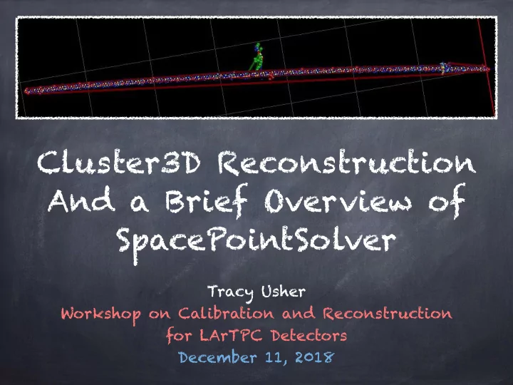
<latexit sha1_base64="2RzcsqSK/LrCgmG8dVPDvaxSgw=">AB6XicdVDLSgNBEOz1GaPRqEcvg0HwtOwGIckt4MVjRNcEkiXMTmaTIbMPZnqFsOQTvHhQ8eqf+Ane/BsnDyGKFjQUVd10dwWpFBod59NaW9/Y3Nou7BR390r7B+XDozudZIpxjyUyUZ2Aai5FzD0UKHknVZxGgeTtYHw589v3XGmRxLc4Sbkf0WEsQsEoGukG+9V+ueLazhzEsRsGtYslabjk26o0S+8ZAYBWv/zRGyQsi3iMTFKtu6Top9ThYJPi32Ms1TysZ0yLuGxjTi2s/np07JmVEGJEyUqRjJXF2dyGmk9SQKTGdEcaR/ezPxL6+bYVj3cxGnGfKYLRaFmSYkNnfZCAUZygnhlCmhLmVsBFVlKFJp7gawv/Eq9oN27k2YdRhgQKcwCmcgws1aMIVtMADBkN4gCd4tqT1aL1Yr4vWNWs5cw/YL19ASyZj2Q=</latexit><latexit sha1_base64="T+rsFLiQNiLJSf5zTl1wKVaC3ls=">AB6XicdVBNS8NAEN3UrxqtVj16WSwFTyEtQtbQRCPFY0tKFstpt26WYTdidCf0JXjyoeBX8If4Eb/4btx9CFX0w8Hhvhpl5QSK4Btf9tHJr6xubW/lte2e3sLdfPDi81XGqKPNoLGLVCYhmgkvmAQfBOoliJAoEawfj85nfvmNK81jewCRhfkSGkoecEjDSNfSr/WKp4rhzYNdpGNTOlqRwd9WqVl4T8sX9lurX/zoDWKaRkwCFUTrbsVNwM+IAk4Fm9q9VLOE0DEZsq6hkRM+9n81CkuG2WAw1iZkoDn6upERiKtJ1FgOiMCI/3bm4l/ed0UwrqfcZmkwCRdLApTgSHGs7/xgCtGQUwMIVRxcyumI6IBZOvRrC/8SrOg3HvTJh1NECeXSMTtApqAaqJL1EIeomiI7tEjerKE9WA9Wy+L1py1nDlCP2C9fgF6qZBf</latexit><latexit sha1_base64="T+rsFLiQNiLJSf5zTl1wKVaC3ls=">AB6XicdVBNS8NAEN3UrxqtVj16WSwFTyEtQtbQRCPFY0tKFstpt26WYTdidCf0JXjyoeBX8If4Eb/4btx9CFX0w8Hhvhpl5QSK4Btf9tHJr6xubW/lte2e3sLdfPDi81XGqKPNoLGLVCYhmgkvmAQfBOoliJAoEawfj85nfvmNK81jewCRhfkSGkoecEjDSNfSr/WKp4rhzYNdpGNTOlqRwd9WqVl4T8sX9lurX/zoDWKaRkwCFUTrbsVNwM+IAk4Fm9q9VLOE0DEZsq6hkRM+9n81CkuG2WAw1iZkoDn6upERiKtJ1FgOiMCI/3bm4l/ed0UwrqfcZmkwCRdLApTgSHGs7/xgCtGQUwMIVRxcyumI6IBZOvRrC/8SrOg3HvTJh1NECeXSMTtApqAaqJL1EIeomiI7tEjerKE9WA9Wy+L1py1nDlCP2C9fgF6qZBf</latexit> Following example event displays utilize the ICARUS TPC simulation/reconstruction
Space point finding works with other TPCs
e.g. was originally developed using MicroBooNE Also handles bad channels ICARUS is a more interesting example because it is a multi-Cryostat and mulit-TPC detector
In the 3D event displays, space points are color coded according to the previously described metric Using a “heat map” - better values of metric are at the red end of the spectrum, worse at the blue end
9
10
Space points color coded using a “heat map” scheme Darker blue means the metric is worse, Darker red means the metric is better Generally you can see that the space points create ribbon-like trajectories (generally) The color coding also illustrates how the quality metric helps visualize the center of the trajectory
11
Zoom to the region where the muon stops and decays to a Michel electron Zoom to the region where a largish delta ray has been produced - worth noting the deviation in the “better” space points in this region
Developed by Chris Backhouse ~Spring/Summer 2017 Goal here is to prefer building of space points from the correct combinations of 2D hits - reduce the level of ambiguity from the simple approach
Starting point is the set of “simple” space points
SpacePointSolver uses different metrics for making initial 3D points
Then try to resolve ambiguous space points using the charge information of the hits
Assume the collection plane charges have the “true” deposition at that time and position Employ a minimization technique to distribute this charge among the matched induction plane hits
Originally motivated by the WireCell though use of 2D hits leads to a different and unique implementation
13
14 Slide content from Chris Backhouse
15 Slide content from Chris Backhouse
16
Monte Carlo Truth
“Simple” Space Points
After Primary Minimization Adding L2 Term
Ambiguous Space Points along a nearly isochronous track
Chris Backhouse has made several presentations
LArSoft Coordinating Meeting August 27, 2017: link Handling bad channels June 8, 2018: link
SpacePointSolver module is implemented in LArSoft with “standard” LArSoft data structures as output
Relatively straightforward to incoporate SpacePointSolver into the Cluster3D framework Which makes it easy to compare against the standard Cluster3D
17
18
Same Event as on Slide 12 Now drawn with Space Points Made with SpacePointSolver Generally, the created Space Points now from a much narrower “ribbon" than those from the simple approach
19
Same zoom perspectives as on slide 13 Chris has continued to develop this with further improvements to the algorithm as well as including the ability to handle bad/dead channels
Surface LArTPCs present two main problems for 2D reconstruction algorithms
Large number of tracks from cosmic ray background means significant volume of data to process - uses significant cpu/ memory Worse, cosmic ray tracks and debris often overlap signal events and require significant special handling - leads to misconstruction and efficiency problems
When viewed in 3D the phase space for overlap is significantly reduced
An algorithm that can look at 3D space points can separate out the information specific to each of the interactions in the TPC Can significantly improve performance - both cpu/memory and
21
Start with a source of 3D hits
Currently either simple or SpacePointSolver
Cluster formation
Initial clustering of space points - DBScan/kdTree Initial “analysis” of the event via Principal Component Analysis Enables Merging “matching” clusters, arbitration of ghost clusters, general cleanup
Resulting clusters represent “slices” of the overall event and the corresponding 2D hits for each slice can now be input to a 2D reconstruction algorithm Important to note that 2D reconstruction algorithms don’ t care about 3D space point ambiguities Note: A similar approach developed by Tingjun using SpacePointSolver for 3D hits, DBScan for clusters, slices then input to TrajCluster
22
The Projection Matching Algorithm (PMA) was originally developed to determine the trajectory of tracks based on 2D hits in each projection
Concept of Principal Curves: here it simultaneously minimizes the projection of a candidate track to hits in each view but, importantly, does not try to get the order of hits correct between the views
It has since been developed to include “micro scale” pattern recognition
Example: given all the hits associated to a CR muon (and its daughters) it should return the CR track trajectory and any delta rays that are also “trackable”.
This is the situation after the first round of clustering with the 3D clustering
All hits associated to a common object are in the “super cluster”, can use the PMA to do the fine level pattern recognition to reconstruct the event Well… this is currently MOSTLY true… some work needs to be done here…
It does not care about ambiguous 3D hits
23
24
Trajectory of PMA Track given by tan colored points Head of PMA Track Note that in a purely “slicing” mode one does not really care about ambiguities - so long as they don’ t merge otherwise independent clusters
25
Focus on this CR
26
Head of PMA track Trajectory of PMA track Worth noting the PMA failures in this event display… this is due to deficiencies in the current interface and hope to be fixed in the future
27
Single isotropic Muon Simulation
Ultimate goal is to have a purely 3D pattern recognition approach to solving the problem The recently rekindled effort in this area has focused on tracking with an idea to create a purely 3D version of the Projection Matching Algorithm
Underlying concept of “principal curves”
This is facilitated by trying to adapt concepts from Computational Geometry:
Principal Components Analysis Convex Hull - making use of defect points Eventually hoping to employ Voronoi diagrams
29
Step 1: Start with a sliced 3D cluster Step 2: Compute the Convex Hull
Computed in 2D by projecting the 3D points into the plane of maximum spread as defined by the Principal Components Analysis
2D for now to facilitate visualization, this should be made 3D in the future
With the hull, use the “defect” points to identify candidate kinks in the trajectory
Use the angle of the two edges to identify kinks
30
31
Simulated Muon in ICARUS
3D Space Points displayed color coded by a measure
“goodness”: darker red - “better” Darker blue - “worse” Principal Components Axes Artificial gap due to distorted waveforms in 2D!
32
Simulated Muon in ICARUS
Project points to plane of maximum spread by PCA, Then compute the convex hull
Ambiguous hits mean kinks can get rounded, kink points ultimately represent centers of interest and will need further investigation Convex Hull Represented by red polygon enclosing cluster Large (sort of) red balls are “defect” points of the convex hull Large yellow balls are kink points on the hull
Now have a gross picture of our cluster
Step 3 is to start breaking it into smaller pieces.
Possible methods:
Break at kink points (if any) Break at defects points with large deviations from the primary PCA Break at “large” gaps If lots of hits simply break in half
Employ a recursive algorithm:
Break cluster by one of the above into two components Recompute PCA, convex hull and find kink points for each Rinse and repeat until “no further gain”
33
34
35
36
PCA & Convex hull
Resulting piecewise linear trajectory
37
Drawing the individual primary principal components axes of the subclusters in a connected fashion Red curve: linked PCA’ s Blue curve: the simulated particle trajectory Note that at this point we have made NO assumptions about the ordering of the 2D Hits
Status and Plans
So far approach seems very promising for developing track trajectories and finding the main kink points This only increases the To Do list:
2D convex hull to 3D, better kink resolution? More powerful computation geometry techniques?
My favorite is Voronoi Diagrams
Refinement of kinks - find actual vertices How will this work for shower reconstruction?
The main problem?
Time, particularly before Deep Learning overwhelms all of this…
38
Two observations
When viewing the event displays it is intriguing to note the path defined by the 3D hits with good (small) values of the metric Also note the density of hits along the particle path
Is there a way to try to “follow” the path more directly?
Can use the end points of the convex hull as path finding end points What might be useful for looking at the density and linking hits together to form a path?
40
In a nutshell - given a set of “site points” the voronoi diagram consists of the collection of voronoi cells, each cell is bounded by the set of points that are equal distance from the interior site point and each of its nearest neighbors Turns out to be very fast to calculate - n log n in the site points What is it good for?
Fast lookup of nearest neighbors Finding high density regions within a given collection of points Can quickly (linear time) get the convex hull Can quickly compute the minimum spanning tree Can use to do “nearest neighbor” averaging…
Investigate if a good starting point for a 3D pattern recognition algorithm
41
Can compute the Voronoi Diagram in the Cluster3D code
Unfortunately, the LArSoft event display has defied all attempts to actually display it!
Previously had explored using the MST in Cluster3D
Followed path using a distance metric but did not handle curvature with ambiguous hits well Using Voronoi Diagram, select nearest neighbor with best metric.
42