
SLIDE 1
Denis Puthier -- BBSG2 2015-2016 -- Denis Puthier -- BBSG2 2015-2016 --
ChIP-seq analysis – D. Puthier
Adapted from “Aviesan Bioinformatic School” (M. Defrance, C. Herrmann, S. Le Gras, J. van Helden, D. Puthier, M. Thomas.Chollier)
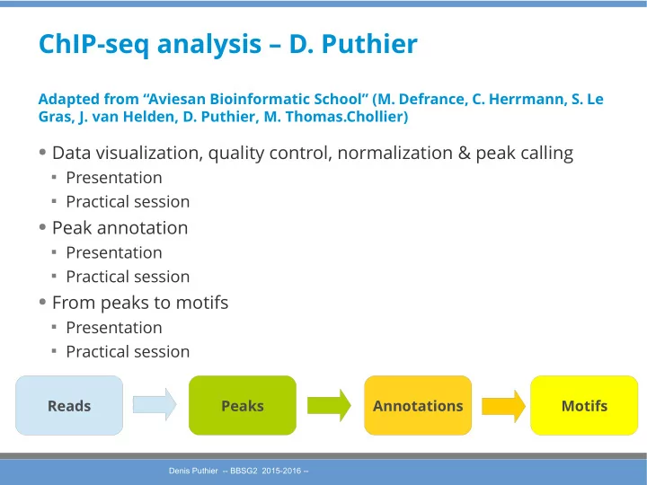
- Data visualization, quality control, normalization & peak calling
Presentation Practical session
- Peak annotation
Presentation Practical session
- From peaks to motifs
Presentation Practical session