Character data Bioinformatics Algorithms (Fundamental Algorithms, - - PDF document

Bioinformatics Algorithms

(Fundamental Algorithms, module 2)

Zsuzsanna Lipt´ ak

Masters in Medical Bioinformatics academic year 2018/19, II semester

Phylogenetics II1

1These slides are partially based on the Lecture Notes from Bielefeld University

”Algorithms for Phylogenetic Reconstruction” (2016/17), by J. Stoye, R. Wittler, et al.

Character data

Now the input data consists of states of characters for the given objects, e.g.

• morphological data, e.g. number of toes, reproductive method, type
• f hip bone, . . . or
• molecular data, e.g. what is the nucletoide in a certain position.

2 / 22

Character data

Example

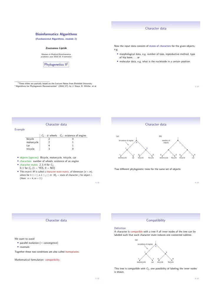
C1 : # wheels C2 : existence of engine bicycle 2 motorcycle 2 1 car 4 1 tricycle 3

• objects (species): Bicycle, motorcycle, tricycle, car
• characters: number of wheels; existence of an engine
• character states: 2, 3, 4 for C1;

0, 1 for C2 (1 = YES, 0 = NO)

• This matrix M is called a character-state-matrix, of dimension (n × m),

where for 1 ≤ i ≤ n, 1 ≤ j ≤ m: Mij = state of character j for object i. (Here: n = 4, m = 2.)

3 / 22

Character data

1

bicycle car tricycle motorcycle invention of engine

(a)

2 2 3 4

number of wheels

(b)

motorcycle car bicycle tricycle

1 1

Two different phylogenetic trees for the same set of objects.

4 / 22

Character data

We want to avoid

• parallel evolution (= convergence)
• reversals

Together these two conditions are also called homoplasies. Mathematical formulation: compatibility.

5 / 22

Compatibility

Definition

A character is compatible with a tree if all inner nodes of the tree can be labeled such that each character state induces one connected subtree.

1

invention of engine

(a)

motorcycle car bicycle tricycle

1 1

This tree is compatible with C2, one possibility of labeling the inner nodes is shown.

6 / 22

Compatibility

Definition

A character is compatible with a tree if all inner nodes of the tree can be labeled such that each character state induces one connected subtree.

bicycle car tricycle motorcycle

2 2 3 4

number of wheels

(b) This tree is compatible with C1. (We have to give a labeling of the inner nodes to prove this.) It is not compatible with C2 (why?)

7 / 22

Compatibility

Definition

A character is compatible with a tree if all inner nodes of the tree can be labeled such that each character state induces one subtree (i.e. is connected).

1

invention of engine

(a)

motorcycle car bicycle tricycle

1 1

This tree is also compatible with C1: We have to give a labeling of the inner nodes (w.r.t. C1) to prove this. (Exercise!)

8 / 22

Compatibility

Here is another example input character-state matrix (here n = 5, m = 2): C1 C2 ↵ A A

• A

C

• C

C

• C

G ✏ G G Our goal is to find a tree that is compatible with every character. Such a tree is called Perfect Phylogeny.

9 / 22

Perfect Phylogeny

Definition

A tree T is called a perfect phylogeny (PP) for C if all characters C ∈ C are compatible with T. Example

AA AC CC CG GG

Why? We have to find a labeling of the inner nodes s.t. for both characters C1 and C2, each state induces a subtree.

10 / 22

Perfect Phylogeny

Definition

A tree T is called a perfect phylogeny (PP) for the character-state matrix M if all characters are compatible with T. Example

AA AC CC CG GG

AC AC CC CG

Note: Our tree (b) for the vehicles was also a PP, since it is compatible both with C1 and with C2.

11 / 22

Perfect Phylogeny

Theorem

Let M be a character-state matrix of dimension n × m, and for 1 ≤ i ≤ m, let ri = number of distinct states in column i (i.e. the number of states which actually occur). Then a tree T is a perfect phylogeny (PP) for M if and only if pc(T) = Pm

i=1(ri − 1).

Example

For the previous example, we have r1 = r2 = 3, so a tree T is a PP iff pc(T) = 2 + 2 = 4.

Example

For the vehicle-example, we have r1 = 2, r2 = 3, therefore if pc(T) = 3, then a tree is a PP.

12 / 22

Perfect Phylogeny

• Ideally, we would like to find a PP for our input data.
• Deciding in general whether a PP exists is NP-hard.

(More precisely: For characters with number of states ≥ 4, the PP problem is NP-hard.)

• Doesn’t really matter, since most of the time, no PP exists anyway.

Why: due to homoplasies; because our input data has errors; our evolutionary model may not be adequate; and, and, and . . .

• Therefore we usually want to find a best possible tree.

13 / 22

Parsimony

Parsimony: What is a best possible tree?

AA AC CC CG GG

AC AC CC CG

Why is this tree “perfect”?

14 / 22

Parsimony

What is a best possible tree?

AA AC CC CG GG

AC AC CC CG

1 1 1 1

Why is this tree “perfect”? Because it has few changes of states!

In red, we marked the edges where there are state changes (an evolutionary event happened), and how many (in this case, always 1).

15 / 22

Parsimony

Definition

The parsimony cost of a phylogenetic tree with labeled inner nodes is the number of state changes along the edges (i.e. the sum of the edge costs, where the cost of an edge = number of characters whose state differs between child and parent).

AA AC CC CG GG

AC AC CC CG

1 1 1 1

The parsimony cost of this labeled tree is 4.

16 / 22

Parsimony

Definition

The parsimony cost of a phylogenetic tree (without labels on the inner nodes) is the minimum of the parsimony cost over all possible labelings of the inner nodes.

AA AC CC CG GG

The parsimony cost of this tree is 4, because the best labeling has cost 4.

17 / 22

Parsimony

Phylogenetic Reconstruction with Character Data

Given a character-state matrix M, our goal is to find a phylogenetic tree which minimizes the parsimony cost. We split the problem into two sub-problems:

• 1. Small Parsimony: Given a phylogenetic tree, find its parsimony cost,

i.e. find a most parsimonious labeling of the inner nodes. This problem can be solved efficiently.

• 2. Large Parsimony or Maximum Parsimony: Find a tree with minimum

parsimony cost. This problem is NP-hard.

18 / 22

Small Parsimony

Small Parsimony Problem

Given: a phylogenetic tree T with character-states at the nodes. Find: a labeling of the inner nodes with states with minimum parsimony cost.

Algorithm

This problem can be solved using Fitch’ algorithm, which runs in time O(nmr), where n = number of species, m = number of characters, and r = maximum number of states over all characters.

19 / 22

Maximum Parsimony

Maximum Parsimony Problem

The maximum parsimony problem is, given a character-state matrix, find a phylogenetic tree with lowest parsimony cost (= a “most parsimonious tree”).

• When a PP exists, then it is also the most parsimonious tree.
• In general, the Maximum Parsimony Problem is NP-hard.

20 / 22

Summary for character data

• When the input is a character-state matrix, then we would like to find

a tree which is compatible with each character.

• Such a tree is called a perfect phylogeny (PP).
• PPP is NP-hard (for number of states ≥ 4).
• Usually, no PP exists, therefore in general . . .
• We are looking for a most parsimonious tree (a tree with lowest

parsimony cost).

• The parsimony cost is defined as the minimum number of the state

changes on the edges over all possible labelings of the inner nodes.

• Recall: There are super-exponentially many trees on n taxa (both

rooted and unrooted), so we cannot try them all.

21 / 22

Summary for character data (cont’ed)

• The problem of finding a most parsimonious tree (a tree with lowest

parsimony cost) is split into Small Parsimony and Maximum Parsimony:

• Small Parsimony can be solved efficienly, e.g. by Fitch’ algorithm.
• Maximum Parsimony is NP-hard, so probably no efficient algorithms

exist.

22 / 22