Chapter 8: Modeling chains of ODEs d R d t = [ r (1 R/K ) bN ] R , - PowerPoint PPT Presentation

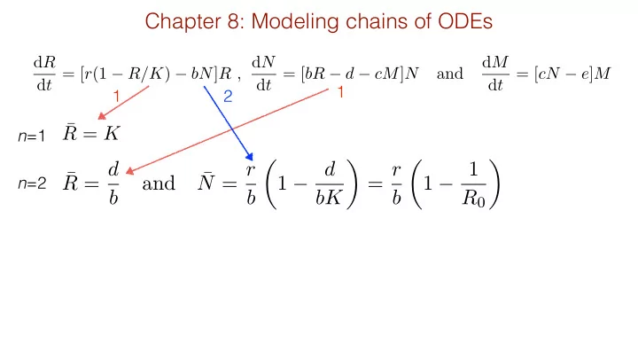
Chapter 8: Modeling chains of ODEs d R d t = [ r (1 − R/K ) − bN ] R , d N d M d t = [ bR − d − cM ] N and d t = [ cN − e ] M , 1 1 2 ¯ R = K n =1 ✓ ◆ ✓ ◆ R = d N = r 1 − d = r 1 − 1 ¯ ¯ and n =2 b b bK b R 0

<latexit sha1_base64="(nul)">(nul)</latexit> <latexit sha1_base64="(nul)">(nul)</latexit> <latexit sha1_base64="(nul)">(nul)</latexit> <latexit sha1_base64="(nul)">(nul)</latexit> Modeling chains of ODEs d R d t = [ r (1 − R/K ) − bN ] R , d N d M d t = [ bR − d − cM ] N and d t = [ cN − e ] M , 3 1 n =1 2 ¯ R = K ✓ ◆ ✓ ◆ R = d N = r 1 − d = r 1 − 1 ¯ ¯ and n =2 b b bK b R 0 0 = cr R 0 be M = b ¯ ✓ ◆ N = e 1 − be R − d ¯ c , ¯ ¯ R = K and n =3 cr c For odd chain lengths R depends on K

Modeling chains of ODEs d R d t = [ r (1 − R/K ) − bN ] R , d N d M d t = [ bR − d − cM ] N and d t = [ cN − e ] M , (a) (b) (c) n =1 n =3 n =2 n =3 M R N ¯ ¯ ¯ n =2 n =3 e d c b 0 0 0 K N K M K N K M K M 0 0 0 K

Kaunzinger & Morin, Nature, 1998 Predator Prey with predator Prey alone Bacterial food chain

<latexit sha1_base64="(nul)">(nul)</latexit> <latexit sha1_base64="(nul)">(nul)</latexit> <latexit sha1_base64="(nul)">(nul)</latexit> <latexit sha1_base64="(nul)">(nul)</latexit> Modeling chains with saturated interaction terms  � d M cN  �  � d R 1 � R bN d N bR cM ⇣ ⌘ N , and d t = h N + N � e M , d t = r R , d t = h R + R � d � � K h R + R h N + N f R : R and N f N : in absence of M no N f M : no M  � d M cN  �  � d R 1 � R bN d N bR cM ⇣ ⌘ N , and d t = h N + N + M � e M d t = r R , d t = h R + R + N � d � � K h R + R + N h N + N + M Per capita function always depends on variable itself. aXY aXY ' when k is large 1 + X/k + Y/k

Modeling chains with Beddington interaction terms (a) (b) (c) n =1 n =3 n =2 n =3 M R ¯ ¯ N ¯ n =2 n =3 e d c b 0 0 0 K N K M K N K M K M 0 0 0 (d) (e) (f) n =3 n =1 n =2 n =2 M R ¯ ¯ N ¯ n =3 n =3 0 K N K N K M 0 K M K M K K K

<latexit sha1_base64="(nul)">(nul)</latexit> <latexit sha1_base64="(nul)">(nul)</latexit> <latexit sha1_base64="(nul)">(nul)</latexit> <latexit sha1_base64="(nul)">(nul)</latexit> Other famous chains don’t suffer from this problem SEIR model: d S d E d I d R d t = s − dS − β SI , d t = β SI − ( d + γ ) E , d t = γ E − ( δ + r ) I and d t = rI − dR S = ( d + γ )( δ + r ) d + γ − d ( δ + r ) γ R = r s ¯ ¯ ¯ ¯ ¯ ¯ I = E = I , E , , δ + r γβ γβ d _ _ R and I are proportional to previous level

<latexit sha1_base64="(nul)">(nul)</latexit> <latexit sha1_base64="(nul)">(nul)</latexit> <latexit sha1_base64="(nul)">(nul)</latexit> <latexit sha1_base64="(nul)">(nul)</latexit> <latexit sha1_base64="(nul)">(nul)</latexit> <latexit sha1_base64="(nul)">(nul)</latexit> <latexit sha1_base64="(nul)">(nul)</latexit> <latexit sha1_base64="(nul)">(nul)</latexit> Cascade of cell divisions d N 0 d N i d N n = s − ( p + d ) N 0 , d t = 2 pN i − 1 − ( p + d ) N i and = 2 pN n − 1 − dN n , d t d t 2 p N n = 2 p s ¯ ¯ ¯ ¯ ¯ N 0 = N i = and p + d , N i − 1 N n − 1 p + d d   − ( p + d ) 0 0 0 0 . . . . . . 2 p − ( p + d ) 0 0 0 . . . . . .     0 2 p − ( p + d ) 0 0 . . . . . . J =   .   .   .   0 0 0 2 p . . . . . . − d ( J 00 − λ )( J 11 − λ )( J 22 − λ ) . . . ( J nn − λ ) = 0

<latexit sha1_base64="(nul)">(nul)</latexit> <latexit sha1_base64="(nul)">(nul)</latexit> <latexit sha1_base64="(nul)">(nul)</latexit> <latexit sha1_base64="(nul)">(nul)</latexit> <latexit sha1_base64="(nul)">(nul)</latexit> <latexit sha1_base64="(nul)">(nul)</latexit> <latexit sha1_base64="(nul)">(nul)</latexit> <latexit sha1_base64="(nul)">(nul)</latexit> Cascade of cell divisions d N 0 d N i d N n = s − ( p + d ) N 0 , d t = 2 pN i − 1 − ( p + d ) N i and = 2 pN n − 1 − dN n , d t d t 2 p N n = 2 p s ¯ ¯ ¯ ¯ ¯ N 0 = N i = and p + d , N i − 1 N n − 1 p + d d ✓ 2 p ◆ n 2 i p i s s N n = s ¯ ¯ ¯ N 0 = N i = and p + d , ( p + d ) i +1 p + d d d Q X d t = − aQ − d Q Q + d f i N i and s = aQ

<latexit sha1_base64="(nul)">(nul)</latexit> <latexit sha1_base64="(nul)">(nul)</latexit> <latexit sha1_base64="(nul)">(nul)</latexit> <latexit sha1_base64="(nul)">(nul)</latexit> <latexit sha1_base64="(null)">(null)</latexit> <latexit sha1_base64="(nul)">(nul)</latexit> <latexit sha1_base64="(nul)">(nul)</latexit> <latexit sha1_base64="(nul)">(nul)</latexit> <latexit sha1_base64="(nul)">(nul)</latexit> <latexit sha1_base64="(null)">(null)</latexit> <latexit sha1_base64="(null)">(null)</latexit> <latexit sha1_base64="(null)">(null)</latexit> Kinetic proofreading Michaelis Menten: d C RL k 1 F + L k − 1 C or d t = k 1 FL − k − 1 C with F = R − C gives C = ⌦ K m + L Kinetic proofreading: k 1 k − 1 k 2 F + L k − 1 C 0 , C i − 1 → C i C i → F and ⌦ d C 0 d C i d C n d t = k 1 FL − ( k − 1 + k 2 ) C 0 , d t = k 2 C i − 1 − ( k − 1 + k 2 ) C i and = k 2 C n − 1 − k − 1 C n d t (8.15) ◆ n n ✓ RL k 2 ¯ X C n = F = R − C i with gives K m + L k − 1 + k 2 i

Kinetic proofreading k 1 k − 1 k 2 F = R − C , F + L k − 1 C 0 , C i − 1 → C i and C i → F , where ⌦ d C 0 d C i d C n d t = k 1 FL − ( k − 1 + k 2 ) C 0 , d t = k 2 C i − 1 − ( k − 1 + k 2 ) C i and = k 2 C n − 1 − k − 1 C n d t (8.15) n =100 n =10 C n > θ ◆ n ✓ RL k 2 log[ L ] ¯ C n = n =0 K m + L k − 1 + k 2 High Low k ∗ − 1 log[ k − 1 ] a ffi nity a ffi nity