Chapter 12: Query Processing Overview Catalog Information for Cost - - PDF document

Chapter 12: Query Processing

• Overview
• Catalog Information for Cost Estimation
• Measures of Query Cost
• Selection Operation
• Sorting
• Join Operation
• Other Operations
• Evaluation of Expressions
• Transformation of Relational Expressions
• Choice of Evaluation Plans

Database Systems Concepts 12.1 Silberschatz, Korth and Sudarshan c 1997

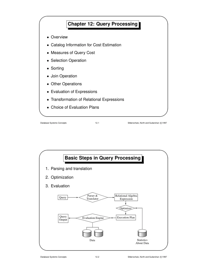
Basic Steps in Query Processing

• 1. Parsing and translation
• 2. Optimization
• 3. Evaluation

Query Parser & Translator Relational Algebra Expression Optimizer Execution Plan Evaluation Engine Query Output Data Statistics About Data

Database Systems Concepts 12.2 Silberschatz, Korth and Sudarshan c 1997

Basic Steps in Query Processing (Cont.)

Parsing and translation

• translate the query into its internal form. This is then translated

into relational algebra.

• Parser checks syntax, verifies relations

Evaluation

• The query-execution engine takes a query-evaluation plan,

executes that plan, and returns the answers to the query.

Database Systems Concepts 12.3 Silberschatz, Korth and Sudarshan c 1997

Basic Steps in Query Processing

Optimization – finding the cheapest evaluation plan for a query.

• Given relational algebra expression may have many equivalent

expressions E.g. σbalance<2500(Πbalance(account)) is equivalent to Πbalance(σbalance<2500(account))

• Any relational-algebra expression can be evaluated in many
• ways. Annotated expression specifying detailed evaluation

strategy is called an evaluation-plan. E.g. can use an index on balance to find accounts with balance < 2500, or can perform complete relation scan and discard accounts with balance ≥ 2500

• Amongst all equivalent expressions, try to choose the one with

cheapest possible evaluation-plan. Cost estimate of a plan based on statistical information in the DBMS catalog.

Database Systems Concepts 12.4 Silberschatz, Korth and Sudarshan c 1997

Catalog Information for Cost Estimation

• nr: number of tuples in relation r.
• br: number of blocks containing tuples of r.
• sr: size of a tuple of r in bytes.
• fr: blocking factor of r — i.e., the number of tuples of r that fit

into one block.

• V(A, r): number of distinct values that appear in r for attribute

A; same as the size of ΠA(r).

• SC(A, r): selection cardinality of attribute A of relation r;

average number of records that satisfy equality on A.

• If tuples of r are stored together physically in a file, then:

br = nr fr

• Database Systems Concepts

12.5 Silberschatz, Korth and Sudarshan c 1997

Catalog Information about Indices

• fi: average fan-out of internal nodes of index i, for

tree-structured indices such as B+-trees.

• HTi: number of levels in index i — i.e., the height of i.

– For a balanced tree index (such as a B+-tree) on attribute A

• f relation r, HTi = ⌈logfi(V(A, r)⌉.

– For a hash index, HTi is 1.

• LBi: number of lowest-level index blocks in i — i.e., the number
• f blocks at the leaf level of the index.

Database Systems Concepts 12.6 Silberschatz, Korth and Sudarshan c 1997

Measures of Query Cost

• Many possible ways to estimate cost, for instance disk

accesses, CPU time, or even communication overhead in a distributed or parallel system.

• Typically disk access is the predominant cost, and is also

relatively easy to estimate. Therefore number of block transfers from disk is used as a measure of the actual cost of evaluation. It is assumed that all transfers of blocks have the same cost.

• Costs of algorithms depend on the size of the buffer in main

memory, as having more memory reduces need for disk

• access. Thus memory size should be a parameter while

estimating cost; often use worst case estimates.

• We refer to the cost estimate of algorithm A as EA. We do not

include cost of writing output to disk.

Database Systems Concepts 12.7 Silberschatz, Korth and Sudarshan c 1997

Selection Operation

• File scan – search algorithms that locate and retrieve records

that fulfill a selection condition.

• Algorithm A1 (linear search). Scan each file block and test all

records to see whether they satisfy the selection condition. – Cost estimate (number of disk blocks scanned) EA1 = br – If selection is on a key attribute, EA1 = (br/ 2) (stop on finding record) – Linear search can be applied regardless of ∗ selection condition, or ∗ ordering of records in the file, or ∗ availability of indices

Database Systems Concepts 12.8 Silberschatz, Korth and Sudarshan c 1997

Selection Operation (Cont.)

• A2 (binary search). Applicable if selection is an equality

comparison on the attribute on which file is ordered. – Assume that the blocks of a relation are stored contiguously – Cost estimate (number of disk blocks to be scanned): EA2 = ⌈log2(br)⌉ + SC(A, r) fr

• − 1

∗ ⌈log2(br)⌉ — cost of locating the first tuple by a binary search on the blocks ∗ SC(A, r) — number of records that will satisfy the selection ∗ ⌈SC(A, r)/fr⌉ — number of blocks that these records will

• ccupy

– Equality condition on a key attribute: SC(A, r) = 1; estimate reduces to EA2 = ⌈log2(br)⌉

Database Systems Concepts 12.9 Silberschatz, Korth and Sudarshan c 1997

Statistical Information for Examples

• faccount = 20

(20 tuples of account fit in one block)

• V(branch-name, account) = 50

(50 branches)

• V(balance, account) = 500

(500 different balance values)

• naccount = 10000

(account has 10,000 tuples)

• Assume the following indices exist on account:

– A primary, B+-tree index for attribute branch-name – A secondary, B+-tree index for attribute balance

Database Systems Concepts 12.10 Silberschatz, Korth and Sudarshan c 1997

Selection Cost Estimate Example

σbranch-name=“Perryridge”(account)

• Number of blocks is baccount = 500: 10, 000 tuples in the

relation; each block holds 20 tuples.

• Assume account is sorted on branch-name.

– V(branch-name, account) is 50 – 10000/ 50 = 200 tuples of the account relation pertain to Perryridge branch – 200/ 20 = 10 blocks for these tuples – A binary search to find the first record would take ⌈log2(500)⌉ = 9 block accesses

• Total cost of binary search is 9 + 10 − 1 = 18 block accesses

(versus 500 for linear scan)

Database Systems Concepts 12.11 Silberschatz, Korth and Sudarshan c 1997

Selections Using Indices

• Index scan – search algorithms that use an index; condition is
• n search-key of index.
• A3 (primary index on candidate key, equality). Retrieve a

single record that satisfies the corresponding equality

• condition. EA3 = HTi + 1
• A4 (primary index on nonkey, equality) Retrieve multiple
• records. Let the search-key attribute be A.

EA4 = HTi +

• SC(A,r)

fr

• A5 (equality on search-key of secondary index).

– Retrieve a single record if the search-key is a candidate key EA5 = HTi + 1 – Retrieve multiple records (each may be on a different block) if the search-key is not a candidate key. EA5 = HTi +SC(A, r)

Database Systems Concepts 12.12 Silberschatz, Korth and Sudarshan c 1997

Cost Estimate Example (Indices)

Consider the query is σbranch-name=“Perryridge”(account), with the primary index on branch-name.

• Since V(branch-name, account) = 50, we expect that

10000/50 = 200 tuples of the account relation pertain to the Perryridge branch.

• Since the index is a clustering index, 200/20 = 10 block reads

are required to read the account tuples

• Several index blocks must also be read. If B+-tree index stores

20 pointers per node, then the B+-tree index must have between 3 and 5 leaf nodes and the entire tree has a depth of

• 2. Therefore, 2 index blocks must be read.
• This strategy requires 12 total block reads.

Database Systems Concepts 12.13 Silberschatz, Korth and Sudarshan c 1997

Selections Involving Comparisons

Implement selections of the form σA≤v(r) or σA≥v(r) by using a linear file scan or binary search, or by using indices in the following ways:

• A6 (primary index, comparison). The cost estimate is:

EA6 = HTi + c fr

• where c is the estimated number of tuples satisfying the
• condition. In absence of statistical information c is assumed to

be nr/ 2.

• A7 (secondary index, comparison). The cost estimate is:

EA7 = HTi + LBi · c nr + c where c is defined as before. (Linear file scan may be cheaper if c is large!)

Database Systems Concepts 12.14 Silberschatz, Korth and Sudarshan c 1997

Implementation of Complex Selections

• The selectivity of a condition θi is the probability that a tuple in

the relation r satisfies θi. If si is the number of satisfying tuples in r, θi’s selectivity is given by si/nr.

• Conjunction: σθ1∧θ2∧...∧θn(r). The estimate for number of

tuples in the result is: nr ∗ s1 ∗ s2 ∗ . . . ∗ sn nn

r

• Disjunction: σθ1∨θ2∨...∨θn(r). Estimated number of tuples:

nr ∗

• 1 − (1 − s1

nr ) ∗ (1 − s2 nr ) ∗ . . . ∗ (1 − sn nr )

• Negation: σ¬θ(r). Estimated number of tuples:

nr − size(σθ(r))

Database Systems Concepts 12.15 Silberschatz, Korth and Sudarshan c 1997

Algorithms for Complex Selections

• A8 (conjunctive selection using one index). Select a

combination of θi and algorithms A1 through A7 that results in the least cost for σθi(r). Test other conditions in memory buffer.

• A9 (conjunctive selection using multiple-key index). Use

appropriate composite (multiple-key) index if available.

• A10 (conjunctive selection by intersection of identifiers).

Requires indices with record pointers. Use corresponding index for each condition, and take intersection of all the

• btained sets of record pointers. Then read file. If some

conditions did not have appropriate indices, apply test in memory.

• A11 (disjunctive selection by union of identifiers). Applicable if

all conditions have available indices. Otherwise use linear scan.

Database Systems Concepts 12.16 Silberschatz, Korth and Sudarshan c 1997

Example of Cost Estimate for Complex Selection

• Consider a selection on account with the following condition:

where branch-name = “Perryridge” and balance = 1200

• Consider using algorithm A8:

– The branch-name index is clustering, and if we use it the cost estimate is 12 block reads ( as we saw before). – The balance index is non-clustering, and V(balance, account) = 500, so the selection would retrieve 10, 000/ 500 = 20 accounts. Adding the index block reads, gives a cost estimate of 22 block reads. – Thus using branch-name index is preferable, even though its condition is less selective. – If both indices were non-clustering, it would be preferable to use the balance index.

Database Systems Concepts 12.17 Silberschatz, Korth and Sudarshan c 1997

Example (cont.)

• Consider using algorithm A10:

– Use the index on balance to retrieve set S1 of pointers to records with balance = 1200. – Use index on branch-name to retrieve set S2 of pointers to records with branch-name = “Perryridge”. – S1 ∩ S2 = set of pointers to records with branch-name = “Perryridge” and balance = 1200. – The number of pointers retrieved (20 and 200) fit into a single leaf page; we read four index blocks to retrieve the two sets of pointers and compute their intersection. – Estimate that one tuple in 50 ∗ 500 meets both conditions. Since naccount = 10000, conservatively overestimate that S1 ∩ S2 contains one pointer. – The total estimated cost of this strategy is five block reads.

Database Systems Concepts 12.18 Silberschatz, Korth and Sudarshan c 1997

Sorting

• We may build an index on the relation, and then use the index

to read the relation in sorted order. May lead to one disk block access for each tuple.

• For relations that fit in memory, techniques like quicksort can

be used. For relations that don’t fit in memory, external sort-merge is a good choice.

Database Systems Concepts 12.19 Silberschatz, Korth and Sudarshan c 1997

External Sort–Merge

Let M denote memory size (in pages).

• 1. Create sorted runs as follows. Let i be 0 initially. Repeatedly

do the following till the end of the relation: (a) Read M blocks of relation into memory (b) Sort the in-memory blocks (c) Write sorted data to run Ri; increment i.

• 2. Merge the runs; suppose for now that i < M. In a single merge

step, use i blocks of memory to buffer input runs, and 1 block to buffer output. Repeatedly do the following until all input buffer pages are empty: (a) Select the first record in sort order from each of the buffers (b) Write the record to the output (c) Delete the record from the buffer page; if the buffer page is empty, read the next block (if any) of the run into the buffer.

Database Systems Concepts 12.20 Silberschatz, Korth and Sudarshan c 1997

Example: External Sorting Using Sort–Merge

g 24 a 19 d 31 c 33 b 14 e 16 r 16 d 21 m 3 p 2 d 7 a 14

• a 14

a 19 b 14 c 33 d 7 d 21 d 31 e 16 g 24 m 3 p 2 r 16

• a 19

b 14 c 33 d 31 e 16 g 24 a 14 d 7 d 21 m 3 p 2 r 16 a 19 d 31 g 24 b 14 c 33 e 16 d 21 m 3 r 16 a 14 d 7 p 2 Initial Relation Create Runs Merge Pass−1 Merge Pass−2 Runs Runs Sorted Output

Database Systems Concepts 12.21 Silberschatz, Korth and Sudarshan c 1997

External Sort–Merge (Cont.)

• If i ≥ M, several merge passes are required.

– In each pass, contiguous groups of M − 1 runs are merged. – A pass reduces the number of runs by a factor of M − 1, and creates runs longer by the same factor. – Repeated passes are performed till all runs have been merged into one.

• Cost analysis:

– Disk accesses for initial run creation as well as in each pass is 2br (except for final pass, which doesn’t write out results) – Total number of merge passes required: ⌈logM−1(br/M)⌉. Thus total number of disk accesses for external sorting: br(2⌈logM−1(br/M)⌉ + 1)

Database Systems Concepts 12.22 Silberschatz, Korth and Sudarshan c 1997

Join Operation

• Several different algorithms to implement joins

– Nested-loop join – Block nested-loop join – Indexed nested-loop join – Merge-join – Hash-join

• Choice based on cost estimate
• Join size estimates required, particularly for cost estimates for
• uter-level operations in a relational-algebra expression.

Database Systems Concepts 12.23 Silberschatz, Korth and Sudarshan c 1997

Join Operation: Running Example

Running example: depositor

Catalog information for join examples:

• ncustomer = 10, 000.
• fcustomer = 25, which implies that

bcustomer = 10000/ 25 = 400.

• ndepositor = 5000.
• fdepositor = 50, which implies that

bdepositor = 5000/ 50 = 100.

• V(customer-name, depositor) = 2500, which implies that, on

average, each customer has two accounts. Also assume that customer-name in depositor is a foreign key on customer.

Database Systems Concepts 12.24 Silberschatz, Korth and Sudarshan c 1997

Estimation of the Size of Joins

• The Cartesian product r × s contains nrns tuples; each tuple
• ccupies sr + ss bytes.
• If R ∩ S = ∅, then r

• If R ∩ S is a key for R, then a tuple of s will join with at most
• ne tuple from r; therefore, the number of tuples in r

greater than the number of tuples in s. If R ∩ S in S is a foreign key in S referencing R, then the number of tuples in r

tuples in s. The case for R ∩ S being a foreign key referencing S is symmetric.

• In the example query depositor

in depositor is a foreign key of customer; hence, the result has exactly ndepositor tuples, which is 5000.

Database Systems Concepts 12.25 Silberschatz, Korth and Sudarshan c 1997

Estimation of the Size of Joins (Cont.)

• If R ∩ S = {A} is not a key for R or S.

If we assume that every tuple t in R produces tuples in R

number of tuples in R

nr ∗ ns V(A, s) If the reverse is true, the estimate obtained will be: nr ∗ ns V(A, r) The lower of these two estimates is probably the more accurate one.

Database Systems Concepts 12.26 Silberschatz, Korth and Sudarshan c 1997

Estimation of the Size of Joins (Cont.)

• Compute the size estimates for depositor

using information about foreign keys: – V(customer-name, depositor) = 2500, and V(customer-name, customer) = 10000 – The two estimates are 5000 ∗ 10000/ 2500 = 20, 000 and 5000 ∗ 10000/ 10000 = 5000 – We choose the lower estimate, which, in this case, is the same as our earlier computation using foreign keys.

Database Systems Concepts 12.27 Silberschatz, Korth and Sudarshan c 1997

Nested-Loop Join

• Compute the theta join, r

for each tuple tr in r do begin for each tuple ts in s do begin test pair (tr, ts) to see if they satisfy the join condition θ if they do, add tr · ts to the result. end end

• r is called the outer relation and s the inner relation of the join.
• Requires no indices and can be used with any kind of join

condition.

• Expensive since it examines every pair of tuples in the two
• relations. If the smaller relation fits entirely in main memory,

use that relation as the inner relation.

Database Systems Concepts 12.28 Silberschatz, Korth and Sudarshan c 1997

Nested-Loop Join (Cont.)

• In the worst case, if there is enough memory only to hold one

block of each relation, the estimated cost is nr ∗ bs + br disk accesses.

• If the smaller relation fits entirely in memory, use that as the

inner relation. This reduces the cost estimate to br + bs disk accesses.

• Assuming the worst case memory availability scenario, cost

estimate will be 5000 ∗ 400 + 100 = 2, 000, 100 disk accesses with depositor as outer relation, and 10000 ∗ 100 + 400 = 1, 000, 400 disk accesses with customer as the outer relation.

• If the smaller relation (depositor) fits entirely in memory, the

cost estimate will be 500 disk accesses.

• Block nested-loops algorithm (next slide) is preferable.

Database Systems Concepts 12.29 Silberschatz, Korth and Sudarshan c 1997

Block Nested-Loop Join

• Variant of nested-loop join in which every block of inner relation

is paired with every block of outer relation. for each block Br of r do begin for each block Bs of s do begin for each tuple tr in Br do begin for each tuple ts in Bs do begin test pair (tr, ts) for satisfying the join condition if they do, add tr · ts to the result. end end end end

• Worst case: each block in the inner relation s is read only once

for each block in the outer relation (instead of once for each tuple in the outer relation)

Database Systems Concepts 12.30 Silberschatz, Korth and Sudarshan c 1997

Block Nested-Loop Join (Cont.)

• Worst case estimate: br ∗ bs + br block accesses. Best case:

br + bs block accesses.

• Improvements to nested-loop and block nested loop

algorithms: – If equi-join attribute forms a key on inner relation, stop inner loop with first match – In block nested-loop, use M − 2 disk blocks as blocking unit for outer relation, where M = memory size in blocks; use remaining two blocks to buffer inner relation and output. Reduces number of scans of inner relation greatly. – Scan inner loop forward and backward alternately, to make use of blocks remaining in buffer (with LRU replacement) – Use index on inner relation if available

Database Systems Concepts 12.31 Silberschatz, Korth and Sudarshan c 1997

Indexed Nested-Loop Join

• If an index is available on the inner loop’s join attribute and join

is an equi-join or natural join, more efficient index lookups can replace file scans.

• Can construct an index just to compute a join.
• For each tuple tr in the outer relation r, use the index to look up

tuples in s that satisfy the join condition with tuple tr.

• Worst case: buffer has space for only one page of r and one

page of the index. – br disk accesses are needed to read relation r, and, for each tuple in r, we perform an index lookup on s. – Cost of the join: br + nr ∗ c, where c is the cost of a single selection on s using the join condition.

• If indices are available on both r and s, use the one with fewer

tuples as the outer relation.

Database Systems Concepts 12.32 Silberschatz, Korth and Sudarshan c 1997

Example of Index Nested-Loop Join

• Compute depositor

relation.

• Let customer have a primary B+-tree index on the join attribute

customer-name, which contains 20 entries in each index node.

• Since customer has 10,000 tuples, the height of the tree is 4,

and one more access is needed to find the actual data.

• Since ndepositor is 5000, the total cost is

100 + 5000 ∗ 5 = 25, 100 disk accesses.

• This cost is lower than the 40, 100 accesses needed for a block

nested-loop join.

Database Systems Concepts 12.33 Silberschatz, Korth and Sudarshan c 1997

Merge–Join

• 1. First sort both relations on their join attribute (if not already

sorted on the join attributes).

• 2. Join step is similar to the merge stage of the sort-merge
• algorithm. Main difference is handling of duplicate values in

join attribute — every pair with same value on join attribute must be matched

a 3 b 1 d 8 d 13 f 7 m 5 q 6 a A b G c L d N m B a1 a2 a1 a3 pr ps r s

Database Systems Concepts 12.34 Silberschatz, Korth and Sudarshan c 1997

Merge–Join (Cont.)

• Each tuple needs to be read only once, and as a result, each

block is also read only once. Thus number of block accesses is br + bs, plus the cost of sorting if relations are unsorted.

• Can be used only for equi-joins and natural joins
• If one relation is sorted, and the other has a secondary B+-tree

index on the join attribute, hybrid merge-joins are possible. The sorted relation is merged with the leaf entries of the B+-tree. The result is sorted on the addresses of the unsorted relation’s tuples, and then the addresses can be replaced by the actual tuples efficiently.

Database Systems Concepts 12.35 Silberschatz, Korth and Sudarshan c 1997

Hash–Join

• Applicable for equi-joins and natural joins.
• A hash function h is used to partition tuples of both relations

into sets that have the same hash value on the join attributes, as follows: – h maps JoinAttrs values to {0, 1, . . . , max}, where JoinAttrs denotes the common attributes of r and s used in the natural join. – Hr0, Hr1, . . . , Hrmax denote partitions of r tuples, each initially

• empty. Each tuple tr ∈ r is put in partition Hri, where

i = h(tr[JoinAttrs]). – Hs0, Hs1, ..., Hsmax denote partitions of s tuples, each initially

• empty. Each tuple ts ∈ s is put in partition Hsi, where

i = h(ts[JoinAttrs]).

Database Systems Concepts 12.36 Silberschatz, Korth and Sudarshan c 1997

Hash–Join (Cont.)

• r tuples in Hri need only to be compared with s tuples in Hsi;

they do not need to be compared with s tuples in any other partition, since: – An r tuple and an s tuple that satisfy the join condition will have the same value for the join attributes. – If that value is hashed to some value i, the r tuple has to be in Hri and the s tuple in Hsi.

Database Systems Concepts 12.37 Silberschatz, Korth and Sudarshan c 1997

Hash–Join (Cont.)

1 2 3 4 1 2 3 4 r s

. . . . . . . .

Partitions

• f r

Partitions

• f s

Database Systems Concepts 12.38 Silberschatz, Korth and Sudarshan c 1997

Hash–Join algorithm

The hash-join of r and s is computed as follows.

• 1. Partition the relations s using hashing function h. When

partitioning a relation, one block of memory is reserved as the

• utput buffer for each partition.
• 2. Partition r similarly.
• 3. For each i:

(a) Load Hsi into memory and build an in-memory hash index

• n it using the join attribute. This hash index uses a

different hash function than the earlier one h. (b) Read the tuples in Hri from disk one by one. For each tuple tr locate each matching tuple ts in Hsi using the in-memory hash index. Output the concatenation of their attributes. Relation s is called the build input and r is called the probe input.

Database Systems Concepts 12.39 Silberschatz, Korth and Sudarshan c 1997

Hash–Join algorithm (Cont.)

• The value max and the hash function h is chosen such that

each Hsi should fit in memory.

• Recursive partitioning required if number of partitions max is

greater than number of pages M of memory. – Instead of partitioning max ways, partition s M − 1 ways; – Further partition the M − 1 partitions using a different hash function – Use same partitioning method on r – Rarely required: e.g., recursive partitioning not needed for relations of 1GB or less with memory size of 2MB, with block size of 4KB.

• Hash-table overflow occurs in partition Hsi if Hsi does not fit in
• memory. Can resolve by further partitioning Hsi using different

hash function. Hri must be similarly partitioned.

Database Systems Concepts 12.40 Silberschatz, Korth and Sudarshan c 1997

Cost of Hash–Join

• If recursive partitioning is not required: 3(br + bs) + 2 ∗ max
• If recursive partitioning is required, number of passes required

for partitioning s is ⌈logM−1(bs) − 1⌉. This is because each final partition of s should fit in memory.

• The number of partitions of probe relation r is the same as that

for build relation s; the number of passes for partitioning of r is also the same as for s. Therefore it is best to choose the smaller relation as the build relation.

• Total cost estimate is:

2(br + bs)⌈logM−1(bs) − 1⌉ + br + bs

• If the entire build input can be kept in main memory, max can

be set to 0 and the algorithm does not partition the relations into temporary files. Cost estimate goes down to br + bs.

Database Systems Concepts 12.41 Silberschatz, Korth and Sudarshan c 1997

Example of Cost of Hash–Join

customer

• Assume that memory size is 20 blocks.
• bdepositor = 100 and bcustomer = 400.
• depositor is to be used as build input. Partition it into five

partitions, each of size 20 blocks. This partitioning can be done in one pass.

• Similarly, partition customer into five partitions, each of size
• 80. This is also done in one pass.
• Therefore total cost: 3(100 + 400) = 1500 block transfers

(Ignores cost of writing partially filled blocks).

Database Systems Concepts 12.42 Silberschatz, Korth and Sudarshan c 1997

Hybrid Hash–Join

• Useful when memory sizes are relatively large, and the build

input is bigger than memory.

• With a memory size of 25 blocks, depositor can be partitioned

into five partitions, each of size 20 blocks.

• Keep the first of the partitions of the build relation in memory. It
• ccupies 20 blocks; one block is used for input, and one block

each is used for buffering the other four partitions.

• customer is similarly partitioned into five partitions each of size

80; the first is used right away for probing, instead of being written out and read back in.

• Ignoring the cost of writing partially filled blocks, the cost is

3(80 + 320) + 20 + 80 = 1300 block transfers with hybrid hash-join, instead of 1500 with plain hash-join.

• Hybrid hash-join most useful if M >> √bs.

Database Systems Concepts 12.43 Silberschatz, Korth and Sudarshan c 1997

Complex Joins

• Join with a conjunctive condition:

r

– Compute the result of one of the simpler joins r

– final result comprises those tuples in the intermediate result that satisfy the remaining conditions θ1 ∧ . . . ∧ θi−1 ∧ θi+1 ∧ . . . ∧ θn – Test these conditions as tuples in r

• Join with a disjunctive condition:

r

Compute as the union of the records in individual joins r

(r

Database Systems Concepts 12.44 Silberschatz, Korth and Sudarshan c 1997

Complex Joins (Cont.)

• Join involving three relations: loan

• Strategy 1. Compute depositor

compute loan

• Strategy 2. Compute loan

result with customer.

• Strategy 3. Perform the pair of joins at once. Build an index on

loan for loan-number, and on customer for customer-name. – For each tuple t in depositor, look up the corresponding tuples in customer and the corresponding tuples in loan. – Each tuple of deposit is examined exactly once.

• Strategy 3 combines two operations into one special-purpose
• peration that is more efficient than implementing two joins of

two relations.

Database Systems Concepts 12.45 Silberschatz, Korth and Sudarshan c 1997

Other Operations

• Duplicate elimination can be implemented via hashing or

sorting. – On sorting duplicates will come adjacent to each other, and all but one of a set of duplicates can be deleted. Optimization: duplicates can be deleted during run generation as well as at intermediate merge steps in external sort-merge. – Hashing is similar – duplicates will come into the same bucket.

• Projection is implemented by performing projection on each

tuple followed by duplicate elimination.

Database Systems Concepts 12.46 Silberschatz, Korth and Sudarshan c 1997

Other Operations (Cont.)

• Aggregation can be implemented in a manner similar to

duplicate elimination. – Sorting or hashing can be used to bring tuples in the same group together, and then the aggregate functions can be applied on each group. – Optimization: combine tuples in the same group during run generation and intermediate merges, by computing partial aggregate values.

• Set operations (∪, ∩ and −): can either use variant of

merge-join after sorting, or variant of hash-join.

Database Systems Concepts 12.47 Silberschatz, Korth and Sudarshan c 1997

Other Operations (Cont.)

• E.g., Set operations using hashing:
• 1. Partition both relations using the same hash function,

thereby creating Hr0, . . ., Hrmax , and Hs0, . . . , Hsmax.

• 2. Process each partition i as follows. Using a different

hashing function, build an in-memory hash index on Hri after it is brought into memory.

• 3. – r ∪ s: Add tuples in Hsi to the hash index if they are not

already in it. Then add the tuples in the hash index to the result. – r ∩ s: output tuples in Hsi to the result if they are already there in the hash index. – r − s: for each tuple in Hsi, if it is there in the hash index, delete it from the index. Add remaining tuples in the hash index to the result.

Database Systems Concepts 12.48 Silberschatz, Korth and Sudarshan c 1997

Other Operations (Cont.)

• Outer join can be computed either as

– A join followed by addition of null-padded non-participating tuples. – by modifying the join algorithms.

• Example:

– In r – –

– Modify merge-join to compute r – –

every tuple tr from r that do not match any tuple in s, output tr padded with nulls. – Right outer-join and full outer-join can be computed similarly.

Database Systems Concepts 12.49 Silberschatz, Korth and Sudarshan c 1997

Evaluation of Expressions

• Materialization: evaluate one operation at a time, starting at

the lowest-level. Use intermediate results materialized into temporary relations to evaluate next-level operations.

• E.g., in figure below, compute and store σbalance<2500(account);

then compute and store its join with customer, and finally compute the projection on customer-name.

Π customer-name σ balance < 2500

account customer

Database Systems Concepts 12.50 Silberschatz, Korth and Sudarshan c 1997

Evaluation of Expressions (Cont.)

• Pipelining: evaluate several operations simultaneously,

passing the results of one operation on to the next.

• E.g., in expression in previous slide, don’t store result of

σbalance<2500(account) – instead, pass tuples directly to the join. Similarly, don’t store result of join, pass tuples directly to projection.

• Much cheaper than materialization: no need to store a

temporary relation to disk.

• Pipelining may not always be possible — e.g., sort, hash-join.
• For pipelining to be effective, use evaluation algorithms that

generate output tuples even as tuples are received for inputs to the operation.

• Pipelines can be executed in two ways: demand driven and

producer driven.

Database Systems Concepts 12.51 Silberschatz, Korth and Sudarshan c 1997

Transformation of Relational Expressions

• Generation of query-evaluation plans for an expression

involves two steps:

• 1. generating logically equivalent expressions
• 2. annotating resultant expressions to get alternative query

plans

• Use equivalence rules to transform an expression into an

equivalent one.

• Based on estimated cost, the cheapest plan is selected. The

process is called cost based optimization.

Database Systems Concepts 12.52 Silberschatz, Korth and Sudarshan c 1997

Equivalence of Expressions

Relations generated by two equivalent expressions have the same set of attributes and contain the same set of tuples, although their attributes may be ordered differently.

Π customer-name

branch depositor

σ branch-city=Brooklyn

account depositor account

σ branch-city=Brooklyn

(a) Initial Expression Tree (b) Transformed Expression Tree branch

Π customer-name

Equivalent expressions

Database Systems Concepts 12.53 Silberschatz, Korth and Sudarshan c 1997

Equivalence Rules

• 1. Conjunctive selection operations can be deconstructed into a

sequence of individual selections. σθ1∧θ2(E) = σθ1(σθ2(E))

• 2. Selection operations are commutative.

σθ1(σθ2(E)) = σθ2(σθ1(E))

• 3. Only the last in a sequence of projection operations is needed,

the others can be omitted. ΠL1(ΠL2(. . . (ΠLn(E)) . . .)) = ΠL1(E)

• 4. Selections can be combined with Cartesian products and theta

joins. (a) σθ(E1 × E2) = E1

(b) σθ1(E1

Database Systems Concepts 12.54 Silberschatz, Korth and Sudarshan c 1997

Equivalence Rules (Cont.)

• 5. Theta-join operations (and natural joins) are commutative.

E1

• 6. (a) Natural join operations are associative:

(E1

(b) Theta joins are associative in the following manner: (E1

where θ2 involves attributes from only E2 and E3.

Database Systems Concepts 12.55 Silberschatz, Korth and Sudarshan c 1997

Equivalence Rules (Cont.)

• 7. The selection operation distributes over the theta join operation

under the following two conditions: (a) When all the attributes in θ0 involve only the attributes of

• ne of the expressions (E1) being joined.

σθ0(E1

(b) When θ1 involves only the attributes of E1 and θ2 involves

• nly the attributes of E2.

σθ1∧θ2(E1

Database Systems Concepts 12.56 Silberschatz, Korth and Sudarshan c 1997

Equivalence Rules (Cont.)

• 8. The projection operation distributes over the theta join
• peration as follows:

(a) if θ involves only attributes from L1 ∪ L2: ΠL1∪L2(E1

(b) Consider a join E1

from E1 and E2, respectively. Let L3 be attributes of E1 that are involved in join condition θ, but are not in L1 ∪ L2, and let L4 be attributes of E2 that are involved in join condition θ, but are not in L1 ∪ L2. ΠL1∪L2(E1

Database Systems Concepts 12.57 Silberschatz, Korth and Sudarshan c 1997

Equivalence Rules (Cont.)

• 9. The set operations union and intersection are commutative

(set difference is not commutative). E1 ∪ E2 = E2 ∪ E1 E1 ∩ E2 = E2 ∩ E1

• 10. Set union and intersection are associative.
• 11. The selection operation distributes over ∪, ∩ and −. E.g.:

σP(E1 − E2) = σP(E1) − σP(E2) For difference and intersection, we also have: σP(E1 − E2) = σP(E1) − E2

• 12. The projection operation distributes over the union operation.

ΠL(E1 ∪ E2) = (ΠL(E1)) ∪ (ΠL(E2))

Database Systems Concepts 12.58 Silberschatz, Korth and Sudarshan c 1997

Selection Operation Example

• Query: Find the names of all customers who have an account

at some branch located in Brooklyn. Πcustomer-name (σbranch-city = “Brooklyn” (branch

• Transformation using rule 7a.

Πcustomer-name ((σbranch-city = “Brooklyn” (branch))

• Performing the selection as early as possible reduces the size
• f the relation to be joined.

Database Systems Concepts 12.59 Silberschatz, Korth and Sudarshan c 1997

Selection Operation Example (Cont.)

• Query: Find the names of all customers with an account at a

Brooklyn branch whose account balance is over $1000. Πcustomer-name (σbranch-city = “Brooklyn” ∧ balance >1000 (branch

• Transformation using join associativity (Rule 6a):

Πcustomer-name ((σbranch-city = “Brooklyn”∧ balance>1000 (branch

• Second form provides an opportunity to apply the “perform

selections early” rule, resulting in the subexpression σbranch-city = “Brooklyn” (branch)

• Thus a sequence of transformations can be useful

Database Systems Concepts 12.60 Silberschatz, Korth and Sudarshan c 1997

Projection Operation Example

Πcustomer-name((σbranch-city = “Brooklyn” (branch)

• When we compute

(σbranch-city = “Brooklyn” (branch)

we obtain a relation whose schema is: (branch-name, branch-city, assets, account-number, balance)

• Push projections using equivalence rules 8a and 8b; eliminate

unneeded attributes from intermediate results to get: Πcustomer-name((Πaccount-number ( (σbranch-city = “Brooklyn” (branch))

Database Systems Concepts 12.61 Silberschatz, Korth and Sudarshan c 1997

Join Ordering Example

• For all relations r1, r2, and r3,

(r1

• If r2

(r1

so that we compute and store a smaller temporary relation.

Database Systems Concepts 12.62 Silberschatz, Korth and Sudarshan c 1997

Join Ordering Example (Cont.)

• Consider the expression

Πcustomer-name ((σbranch-city = “Brooklyn” (branch))

• Could compute account

σbranch-city = “Brooklyn” (branch) but account

• Since it is more likely that only a small fraction of the bank’s

customers have accounts in branches located in Brooklyn, it is better to compute σbranch-city = “Brooklyn” (branch)

first.

Database Systems Concepts 12.63 Silberschatz, Korth and Sudarshan c 1997

Evaluation Plan

An evaluation plan defines exactly what algorithm is used for each

• peration, and how the execution of the operations is coordinated.

σ branch-city=Brooklyn

branch

Π customer-name (sort to remove duplicates)

account depositor

σ balance < 1000

(use index 1) (use linear scan) (hash-join) (merge-join) Pipeline Pipeline

An evaluation plan

Database Systems Concepts 12.64 Silberschatz, Korth and Sudarshan c 1997

Choice of Evaluation Plans

• Must consider the interaction of evaluation techniques when

choosing evaluation plans: choosing the cheapest algorithm for each operation independently may not yield the best overall

• algorithm. E.g.

– merge-join may be costlier than hash-join, but may provide a sorted output which reduces the cost for an outer level aggregation. – nested-loop join may provide opportunity for pipelining

• Practical query optimizers incorporate elements of the

following two broad approaches:

• 1. Search all the plans and choose the best plan in a

cost-based fashion.

• 2. Use heuristics to choose a plan.

Database Systems Concepts 12.65 Silberschatz, Korth and Sudarshan c 1997

Cost-Based Optimization

• Consider finding the best join-order for r1

• There are (2(n − 1))!/ (n − 1)! different join orders for above
• expression. With n = 7, the number is 665280, with n = 10, the

number is greater than 176 billion!

• No need to generate all the join orders. Using dynamic

programming, the least-cost join order for any subset of {r1, r2, . . ., rn} is computed only once and stored for future use.

• This reduces time complexity to around O(3n). With n = 10,

this number is 59000.

Database Systems Concepts 12.66 Silberschatz, Korth and Sudarshan c 1997

Cost-Based Optimization (Cont.)

• In left-deep join trees, the right-hand-side input for each join

is a relation, not the result of an intermediate join.

• If only left-deep join trees are considered, cost of finding best

join order becomes O(2n).

r4 r5 r3 r1 r2 r5 r4 r3 r2 r1 (a) Left-deep Join Tree (b) Non-left-deep Join Tree

Database Systems Concepts 12.67 Silberschatz, Korth and Sudarshan c 1997

Dynamic Programming in Optimization

• To find best left-deep join tree for a set of n relations:

– Consider n alternatives with one relation as right-hand-side input and the other relations as left-hand-side input. – Using (recursively computed and stored) least-cost join

• rder for each alternative on left-hand-side, choose the

cheapest of the n alternatives.

• To find best join tree for a set of n relations:

– To find best plan for a set S of n relations, consider all possible plans of the form: S1

non-empty subset of S. – As before, use recursively computed and stored costs for subsets of S to find the cost of each plan. Choose the cheapest of the 2n − 1 alternatives.

Database Systems Concepts 12.68 Silberschatz, Korth and Sudarshan c 1997

Interesting Orders in Cost-Based Optimization

• Consider the expression (r1

• An interesting sort order is a particular sort order of tuples

that could be useful for a later operation. – Generating the result of r1

common with r4 or r5 may be useful, but generating it sorted

• n the attributes common to only r1 and r2 is not useful.

– Using merge–join to compute r1

but may provide an output sorted in an interesting order.

• Not sufficient to find the best join order for each subset of the

set of n given relations; must find the best join order for each subset, for each interesting sort order of the join result for that

• subset. Simple extension of earlier dynamic programming

algorithms.

Database Systems Concepts 12.69 Silberschatz, Korth and Sudarshan c 1997

Heuristic Optimization

• Cost-based optimization is expensive, even with dynamic

programming.

• Systems may use heuristics to reduce the number of choices

that must be made in a cost-based fashion.

• Heuristic optimization transforms the query-tree by using a set
• f rules that typically (but not in all cases) improve execution

performance: – Perform selection early (reduces the number of tuples) – Perform projection early (reduces the number of attributes) – Perform most restrictive selection and join operations before other similar operations.

• Some systems use only heuristics, others combine heuristics

with partial cost-based optimization.

Database Systems Concepts 12.70 Silberschatz, Korth and Sudarshan c 1997

Steps in Typical Heuristic Optimization

• 1. Deconstruct conjunctive selections into a sequence of single

selection operations (Equiv. rule 1).

• 2. Move selection operations down the query tree for the earliest

possible execution (Equiv. rules 2, 7a, 7b, 11).

• 3. Execute first those selection and join operations that will

produce the smallest relations (Equiv. rule 6).

• 4. Replace Cartesian product operations that are followed by a

selection condition by join operations (Equiv. rule 4a).

• 5. Deconstruct and move as far down the tree as possible lists of

projection attributes, creating new projections where needed (Equiv. rules 3, 8a, 8b, 12).

• 6. Identify those subtrees whose operations can be pipelined,

and execute them using pipelining.

Database Systems Concepts 12.71 Silberschatz, Korth and Sudarshan c 1997

Structure of Query Optimizers

• The System R optimizer considers only left-deep join orders.

This reduces optimization complexity and generates plans amenable to pipelined evaluation. System R also uses heuristics to push selections and projections down the query tree.

• For scans using secondary indices, the Sybase optimizer takes

into account the probability that the page containing the tuple is in the buffer.

Database Systems Concepts 12.72 Silberschatz, Korth and Sudarshan c 1997

Structure of Query Optimizers (Cont.)

• Some query optimizers integrate heuristic selection and the

generation of alternative access plans. – System R and Starburst use a hierarchical procedure based

• n the nested-block concept of SQL: heuristic rewriting

followed by cost-based join-order optimization. – The Oracle7 optimizer supports a heuristic based on available access paths.

• Even with the use of heuristics, cost-based query optimization

imposes a substantial overhead. This expense is usually more than offset by savings at query-execution time, particularly by reducing the number of slow disk accesses.

Database Systems Concepts 12.73 Silberschatz, Korth and Sudarshan c 1997