Ch 8/9: Spatial Data, Networks marks for previous 2 weeks published - - PowerPoint PPT Presentation

ch 8 9 spatial data networks
SMART_READER_LITE
LIVE PREVIEW

Ch 8/9: Spatial Data, Networks marks for previous 2 weeks published - - PowerPoint PPT Presentation

News Arrange spatial data Ch 8/9: Spatial Data, Networks marks for previous 2 weeks published Use Given Geometry first week was pass/fail for having anything Paper: Genealogical Graphs Geographic now more fine-grained guidance


slide-1
SLIDE 1

www.cs.ubc.ca/~tmm/courses/547-17F

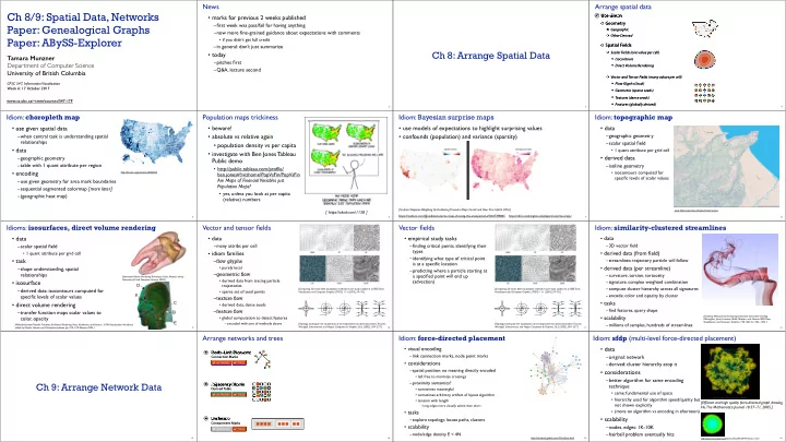
Ch 8/9: Spatial Data, Networks Paper: Genealogical Graphs Paper: ABySS-Explorer

Tamara Munzner Department of Computer Science University of British Columbia

CPSC 547, Information Visualization Week 6: 17 October 2017

News

  • marks for previous 2 weeks published

–first week was pass/fail for having anything –now more fine-grained guidance about expectations with comments

  • if you didn’t get full credit

–in general: don’t just summarize

  • today

–pitches first –Q&A, lecture second

2

Ch 8: Arrange Spatial Data

3 4

Arrange spatial data

Use Given Geometry

Geographic Other Derived

Spatial Fields

Scalar Fields (one value per cell) Isocontours Direct Volume Rendering Vector and Tensor Fields (many values per cell) Flow Glyphs (local) Geometric (sparse seeds) Textures (dense seeds) Features (globally derived)

Idiom: choropleth map

  • use given spatial data

–when central task is understanding spatial relationships

  • data

–geographic geometry –table with 1 quant attribute per region

  • encoding

–use given geometry for area mark boundaries –sequential segmented colormap [more later] –(geographic heat map)

5

http://bl.ocks.org/mbostock/4060606

Population maps trickiness

  • beware!
  • absolute vs relative again
  • population density vs per capita
  • investigate with Ben Jones Tableau

Public demo

  • http://public.tableau.com/profile/

ben.jones#!/vizhome/PopVsFin/PopVsFin
 Are Maps of Financial Variables just Population Maps?

  • yes, unless you look at per capita

(relative) numbers

6

[ https://xkcd.com/1138 ]

Idiom: Bayesian surprise maps

  • use models of expectations to highlight surprising values
  • confounds (population) and variance (sparsity)

7

[Surprise! Bayesian Weighting for De-Biasing Thematic Maps. Correll and Heer. Proc InfoVis 2016] https://medium.com/@uwdata/surprise-maps-showing-the-unexpected-e92b67398865 https://idl.cs.washington.edu/papers/surprise-maps/

Idiom: topographic map

  • data

–geographic geometry –scalar spatial field

  • 1 quant attribute per grid cell
  • derived data

–isoline geometry

  • isocontours computed for

specific levels of scalar values

8

Land Information New Zealand Data Service

Idioms: isosurfaces, direct volume rendering

  • data

–scalar spatial field

  • 1 quant attribute per grid cell
  • task

–shape understanding, spatial relationships

  • isosurface

–derived data: isocontours computed for specific levels of scalar values

  • direct volume rendering

–transfer function maps scalar values to color, opacity

9

[Interactive Volume Rendering

  • Techniques. Kniss. Master’s thesis,

University of Utah Computer Science, 2002.] [Multidimensional Transfer Functions for Volume Rendering. Kniss, Kindlmann, and Hansen. In The Visualization Handbook, edited by Charles Hansen and Christopher Johnson, pp. 189–210. Elsevier, 2005.]

B C E D F

Vector and tensor fields

  • data

–many attribs per cell

  • idiom families

–flow glyphs

  • purely local

–geometric flow

  • derived data from tracing particle

trajectories

  • sparse set of seed points

–texture flow

  • derived data, dense seeds

–feature flow

  • global computation to detect features

– encoded with one of methods above

10

[Comparing 2D vector field visualization methods: A user study. Laidlaw et al. IEEE Trans. Visualization and Computer Graphics (TVCG) 11:1 (2005), 59–70.] [Topology tracking for the visualization of time-dependent two-dimensional flows. Tricoche, Wischgoll, Scheuermann, and Hagen. Computers & Graphics 26:2 (2002), 249–257.]

Vector fields

  • empirical study tasks

–finding critical points, identifying their types –identifying what type of critical point is at a specific location –predicting where a particle starting at a specified point will end up (advection)

11

[Comparing 2D vector field visualization methods: A user study. Laidlaw et al. IEEE Trans. Visualization and Computer Graphics (TVCG) 11:1 (2005), 59–70.] [Topology tracking for the visualization of time-dependent two-dimensional flows. Tricoche, Wischgoll, Scheuermann, and Hagen. Computers & Graphics 26:2 (2002), 249–257.]

Idiom: similarity-clustered streamlines

  • data

–3D vector field

  • derived data (from field)

–streamlines: trajectory particle will follow

  • derived data (per streamline)

–curvature, torsion, tortuosity –signature: complex weighted combination –compute cluster hierarchy across all signatures –encode: color and opacity by cluster

  • tasks

–find features, query shape

  • scalability

–millions of samples, hundreds of streamlines

12

[Similarity Measures for Enhancing Interactive Streamline Seeding. McLoughlin,. Jones, Laramee, Malki, Masters, and. Hansen. IEEE Trans. Visualization and Computer Graphics 19:8 (2013), 1342–1353.]

Ch 9: Arrange Network Data

13 14

Arrange networks and trees

Node–Link Diagrams Enclosure Adjacency Matrix

TREES NETWORKS

Connection Marks

TREES NETWORKS

Derived Table

TREES NETWORKS

Containment Marks

Idiom: force-directed placement

  • visual encoding

–link connection marks, node point marks

  • considerations

–spatial position: no meaning directly encoded

  • left free to minimize crossings

–proximity semantics?

  • sometimes meaningful
  • sometimes arbitrary, artifact of layout algorithm
  • tension with length

– long edges more visually salient than short

  • tasks

–explore topology; locate paths, clusters

  • scalability

–node/edge density E < 4N

15

http://mbostock.github.com/d3/ex/force.html

Idiom: sfdp (multi-level force-directed placement)

  • data

–original: network –derived: cluster hierarchy atop it

  • considerations

–better algorithm for same encoding technique

  • same: fundamental use of space
  • hierarchy used for algorithm speed/quality but

not shown explicitly

  • (more on algorithm vs encoding in afternoon)
  • scalability

–nodes, edges: 1K-10K –hairball problem eventually hits

16

[Efficient and high quality force-directed graph drawing. Hu. The Mathematica Journal 10:37–71, 2005.]

http://www.research.att.com/yifanhu/GALLERY/GRAPHS/index1.html

slide-2
SLIDE 2

Idiom: adjacency matrix view

  • data: network

–transform into same data/encoding as heatmap

  • derived data: table from network

–1 quant attrib

  • weighted edge between nodes

–2 categ attribs: node list x 2

  • visual encoding

–cell shows presence/absence of edge

  • scalability

–1K nodes, 1M edges

17

[NodeTrix: a Hybrid Visualization of Social Networks. Henry, Fekete, and McGuffin. IEEE TVCG (Proc. InfoVis) 13(6):1302-1309, 2007.] [Points of view: Networks. Gehlenborg and

  • Wong. Nature Methods 9:115.]

Connection vs. adjacency comparison

  • adjacency matrix strengths

–predictability, scalability, supports reordering –some topology tasks trainable

  • node-link diagram strengths

–topology understanding, path tracing –intuitive, no training needed

  • empirical study

–node-link best for small networks –matrix best for large networks

  • if tasks don’t involve topological structure!

18

[On the readability of graphs using node-link and matrix-based representations: a controlled experiment and statistical analysis. Ghoniem, Fekete, and Castagliola. Information Visualization 4:2 (2005), 114–135.]

http://www.michaelmcguffin.com/courses/vis/patternsInAdjacencyMatrix.png

Idiom: radial node-link tree

  • data

–tree

  • encoding

–link connection marks –point node marks –radial axis orientation

  • angular proximity: siblings
  • distance from center: depth in tree
  • tasks

–understanding topology, following paths

  • scalability

–1K - 10K nodes

19

http://mbostock.github.com/d3/ex/tree.html

!"#$ " % " & ' ( ) * + *&,+($#

  • ..&/0$#"()1$2&,+($#

2/00,%)('3(#,*(,#$ 4)$#"#*5)*"&2&,+($# 6 $ # . $ 7 8 . $ . # " 9 5 : $ ( ; $ $ % % $ + + 2 $ % ( # " & ) ( ' < ) % = > ) + ( " % * $ 6 " ? @ & / ; 6 ) % 2 , ( 35/#($+(A"(5+ 39"%%)%.B#$$ /9()0)C"()/%

  • +9$*(D"()/:"%=$#

"%)0"($ 7 " + ) % . @,%*()/%3$E,$%*$ ) % ( $ # 9 / & " ( $

  • #

# " ' F % ( $ # 9 / & " ( / # 2 / & / # F % ( $ # 9 / & " ( / # > " ( $ F % ( $ # 9 / & " ( / # F%($#9/&"(/# 6 " ( # ) ? F % ( $ # 9 / & " ( / # G , H $ # F % ( $ # 9 / & " ( / # IHJ$*(F%($#9/&"(/# A / ) % ( F % ( $ # 9 / & " ( / # D$*("%.&$F%($#9/&"(/# F3*5$8,&"H&$ A " # " & & $ & A",+$ 3*5$8,&$# 3$E,$%*$ B # " % + ) ( ) / % B # " % + ) ( ) / % $ # B#"%+)()/%71$%( B;$$% 8 " ( " */%1$#($#+ 2/%1$#($#+ >$&)0)($8B$?(2/%1$#($# K#"956<2/%1$#($# F>"("2/%1$#($# L3IG2/%1$#($# > " ( " @ ) $ & 8 > " ( " 3 * 5 $ " > " ( " 3 $ ( >"("3/,#*$ >"("B"H&$ >"("M()& 8)+9&"' >)#('39#)($ <)%$39#)($ D$*(39#)($ B $ ? ( 3 9 # ) ( $ ! $ ? @ & " # $ N ) + 9 5 ' + ) * + >#".@/#*$ K#"1)('@/#*$ F@/#*$ G:/8'@/#*$ A " # ( ) * & $ 3)0,&"()/% 3 9 # ) % . 39#)%.@/#*$ E , $ # '

  • ..#$."($7?9#$++)/%
  • %8
  • #

) ( 5 $ ( ) *

  • 1$#".$

:)%"#'7?9#$++)/% 2/09"#)+/% 2 / 9 / + ) ( $ 7 ? 9 # $ + + ) / % 2 / , % ( >"($M()& >)+()%*( 7 ? 9 # $ + + ) / % 7?9#$++)/%F($#"(/# @% FO F +

  • <)($#"&

6 " ( * 5 6"?)0,0 0$(5/8+ " 8 8 "%8 "1$#".$ */,%( 8)+()%*( 8)1 $E O% .( .($ )OO )+" &( &($ 0"? 0)% 0/8 0,& %$E %/( / # / # 8 $ # H ' #"%.$ + $ & $ * ( + ( 8 8 $ 1 +,H +,0 , 9 8 " ( $ 1"#)"%*$ ;5$#$ ? / # P 6)%)0,0 G/( I # Q , $ # ' D " % . $ 3 ( # ) % . M ( ) & 3,0 N"#)"H&$ N"#)"%*$ R/# +*"&$ F 3 * " & $ 6 " 9 <)%$"#3*"&$ < / . 3 * " & $ I#8)%"&3*"&$ Q , " % ( ) & $ 3 * " & $ Q,"%()("()1$3*"&$ D / / ( 3 * " & $ 3*"&$ 3*"&$B'9$ B)0$3*"&$ ,()&

  • ##"'+

2/&/#+ >"($+ > ) + 9 & " ' + @)&($# K$/0$(#' 5$"9 @)H/%"**)4$"9 4 $ " 9 G / 8 $ F 7 1 " & , " H & $ FA#$8)*"($ FN"&,$A#/?' 0"(5 >$%+$6"(#)? F6"(#)? 3 9 " # + $ 6 " ( # ) ? 6"(5+ I#)$%("()/% 9"&$(($ 2/&/#A"&$(($ A"&$(($ 35"9$A"&$(($ 3)C$A"&$(($ A#/9$#(' 35"9$+ 3 / # ( 3 ( " ( + 3 ( # ) % . + 1)+ " ? ) +

  • ?$+
  • ?)+
  • ?

) + K # ) 8 < ) % $

  • ?

) + < " H $ & 2"#($+)"%-?$+ * / % ( # / & +

  • %

* 5 / # 2 / % ( # / & 2 & ) * = 2 / % ( # / & 2 / % ( # / & 2/%(#/&<)+( > # " . 2 / % ( # / & 7 ? 9 " % 8 2 / % ( # / & 4/1$#2/%(#/& F2/%(#/& A " % S / / 2 / % ( # / & 3$&$*()/%2/%(#/& B//&()92/%(#/& 8 " ( " >"(" >"("<)+( >"("39#)($ 78.$39#)($ G / 8 $ 3 9 # ) ( $ #$%8$#

  • ##/;B'9$

7 8 . $ D $ % 8 $ # $ # FD$%8$#$# 3 5 " 9 $ D $ % 8 $ # $ # 3 * " & $ : ) % 8 ) % . B # $ $ B#$$:,)&8$# $1$%(+ > " ( " 7 1 $ % ( 3 $ & $ * ( ) / % 7 1 $ % ( B / / & ( ) 9 7 1 $ % ( N)+,"&)C"()/%71$%( & $ . $ % 8 <$.$%8 < $ . $ % 8 F ( $ < $ . $ % 8 D " % . $ /9$#"(/# 8)+(/#()/% :)O/*"&>)+(/#()/% >)+(/#()/% @)+5$'$>)+(/#()/% $%*/8$# 2/&/#7%*/8$# 7 % * / 8 $ # A#/9$#('7%*/8$# 35"9$7%*/8$# 3)C$7%*/8$# T&($# @)+5$'$B#$$@)&($# K#"95>)+("%*$@)&($# N ) + ) H ) & ) ( ' @ ) & ( $ # F I 9 $ # " ( / # &"H$& <"H$&$# D"8)"&<"H$&$# 3("*=$8-#$"<"H$&$# & " ' / , (

  • ?)+<"'/,(

:,%8&$878.$D/,($# 2 ) # * & $ < " ' / , ( 2)#*&$A"*=)%.<"'/,( >$%8#/.#"0<"'/,( @ / # * $ > ) # $ * ( $ 8 < " ' / , ( F * ) * & $ B # $ $ < " ' / , ( F % 8 $ % ( $ 8 B # $ $ < " ' / , ( <"'/,( G / 8 $ < ) % = B # $ $ < " ' / , ( A ) $ < " ' / , ( D"8)"&B#$$<"'/,( D"%8/0<"'/,( 3 ( " * = $ 8

  • #

$ " < " ' / , ( B#$$6"9<"'/,( I 9 $ # " ( / # I 9 $ # " ( / # < ) + ( I9$#"(/#3$E,$%*$ I9$#"(/#3;)(*5 3/#(I9$#"(/# N ) + , " & ) C " ( ) / %

Idiom: treemap

  • data

–tree –1 quant attrib at leaf nodes

  • encoding

–area containment marks for hierarchical structure –rectilinear orientation –size encodes quant attrib

  • tasks

–query attribute at leaf nodes

  • scalability

–1M leaf nodes

20

http://www.nytimes.com/packages/html/newsgraphics/2011/0119-budget/index.html

Link marks: Connection and containment

  • marks as links (vs. nodes)

–common case in network drawing –1D case: connection

  • ex: all node-link diagrams
  • emphasizes topology, path tracing
  • networks and trees

–2D case: containment

  • ex: all treemap variants
  • emphasizes attribute values at leaves (size

coding)

  • only trees

21

Node–Link Diagram Treemap

[Elastic Hierarchies: Combining Treemaps and Node-Link

  • Diagrams. Dong, McGuffin, and Chignell. Proc. InfoVis

2005, p. 57-64.]

Containment Connection

Tree drawing idioms comparison

  • data shown

– link relationships – tree depth – sibling order

  • design choices

– connection vs containment link marks – rectilinear vs radial layout – spatial position channels

  • considerations

– redundant? arbitrary? – information density?

  • avoid wasting space

22

[Quantifying the Space-Efficiency of 2D Graphical Representations of

  • Trees. McGuffin and Robert. Information

Visualization 9:2 (2010), 115–140.]

Paper: Genealogical Graphs

23

Genealogical graphs: Technique paper

  • family tree is a misnomer

–single person has tree of ancestors, tree of descendants –pedigree collapse inevitable

  • diamond in ancestor graph
  • crowding problem

–exponential

  • fractal layout

–poor info density –no spatial ordering for generations

24

[Fig 2, 6, 7. Interactive Visualization of Genealogical Graphs. Michael J. McGuffin, Ravin Balakrishnan. Proc. InfoVis 2005, pp 17-24.]

Layouts

  • rooted trees: standard layouts

–connection –containment –adjacent aligned position –indented position

25

[Fig 8. Interactive Visualization of Genealogical Graphs. Michael J. McGuffin, Ravin Balakrishnan. Proc. InfoVis 2005, pp 17-24.]

Layouts

  • free trees

–no root

  • adapting rooted methods

–temporary root for given focus –containment (nested)

26

[Fig 9. Interactive Visualization of Genealogical Graphs. Michael J. McGuffin, Ravin Balakrishnan. Proc. InfoVis 2005, pp 17-24.]

Dual trees abstraction

  • explore canonical subsets and combinations, easy to interpret, scales well
  • no crossings, nodes ordered by generation
  • doubly rooted: x leftmost descend, y rightmost ancestor

–offset roots from hourglass diagram

27

[Fig 10. Interactive Visualization of Genealogical Graphs. Michael J. McGuffin, Ravin Balakrishnan. Proc. InfoVis 2005, pp 17-24.]

Indented, flipped, combined

28

[Fig 11. Interactive Visualization of Genealogical Graphs. Michael J. McGuffin, Ravin Balakrishnan. Proc. InfoVis 2005, pp 17-24.]

Another example

  • vertical connection
  • horizontal connection
  • indented
  • upcoming chapters

–layering –aggregation

29

[Fig 13. Interactive Visualization of Genealogical Graphs. Michael J. McGuffin, Ravin Balakrishnan. Proc. InfoVis 2005, pp 17-24.]

Interaction as fundamental to design

  • navigation

–topological navigation via collapse/expand on selection

  • parents, children
  • expand can trigger rotation

– collapsing others – layout driven by navigation

–geometric zoom/pan –constrained navigation: automatic camera framing

  • animated transitions

–3 phases: fade out, move, fade in

  • mouseover hover

–preview dots: expand if collapsed

30

[Fig 14. Interactive Visualization of Genealogical Graphs. Michael J. McGuffin, Ravin Balakrishnan. Proc. InfoVis 2005, pp 17-24.]

Custom widget

  • popup marking menu

–flick up or down, ballistic –subtree drag-out widget

31

[Fig 14. Interactive Visualization of Genealogical Graphs. Michael J. McGuffin, Ravin Balakrishnan. Proc. InfoVis 2005, pp 17-24.]

Paper: ABySS-Explorer

32

slide-3
SLIDE 3

ABySS-Explorer: Design study

  • reconstructing genome with ABySS algorithm


(Assembly By Short Sequences)

  • domain task

–go from short subsequences to contigs, long contiguous sequences –extensive automatic support, but still human in the loop for visual inspection and manual editing –ambiguities, like repetitions longer than read length

  • data, domain:abstract

–millions of reads of 25-100 nucleotides (nt): strings –read coverage, proxy for quality: quant attrib –read pairing distances, proxy for size distribution: quant

33

Fig 2. ABySS-Explorer: visualizing genome sequence assemblies. Nielsen, Jackman, Birol, Jones. TVCG 15(6):881-8, 2009 (Proc. InfoVis 2009).

Contigs: abstraction as derived network data

  • derived data: de Bruijn graph/network

–directed network, compact representation of sequence overlaps –node: contig –edge: overlap of k − 1 nt between two contigs –good for computing, bad for reasoning about sequence space

  • derived data: dual de Bruijn graph

–node: points of contig overlap –edge: contig –better match for arrow diagrams used in hand drawn sketches

  • base layout: force-directed

34

Fig 3. ABySS-Explorer: visualizing genome sequence assemblies. Nielsen, Jackman, Birol, Jones. TVCG 15(6):881-8, 2009 (Proc. InfoVis 2009).

DNA as double stranded: idiom for encoding & interaction

  • rejected option: 2 nodes per contig

–excess clutter if one for each direction –choice at data abstraction level

  • encoding & interaction idiom: polar node

–encoding: upper vs lower attachment point

  • redundant with arc direction

– large-scale visibility, without need to zoom

  • arbitrary but consistent

–interaction: click to reverse direction

  • switches polarity of vertex connections
  • changes sign of label

35

Fig 4. ABySS-Explorer: visualizing genome sequence assemblies. Nielsen, Jackman, Birol, Jones. TVCG 15(6):881-8, 2009 (Proc. InfoVis 2009).

Contig length: encoding

  • rejected option: scale edge lengths by sequence lengths

–short contigs are important sources of ambiguity, would be hard to distinguish –task guidance: only low-res judgements needed, relatively long or short

  • encoding idiom: wave pattern

–oscillation shows fixed number, shapes distinguishable –min amplitude at connections so edges visible –orientation with max amplitude asymmetric wrt start

  • rejected initial option: max in middle
  • rejected options:

– color (keep for other attribute) – half-lines – curvature (used for polar nodes)

  • aligned with empirical guidance for tapered edges

36

Fig 5. ABySS-Explorer: visualizing genome sequence assemblies. Nielsen, Jackman, Birol, Jones. TVCG 15(6):881-8, 2009 (Proc. InfoVis 2009). 12K nt 3K nt

Contig coverage: encoding

  • rejected options: luminance/lightness

–not distinguishable given denseness variation from wave shapes –also problematic with desire for separable color/hue encoding

  • chosen: line thickness

–not distinguishable for extremely long contigs –can address by adjusting oscillation frequency to suitable size

37

Read pairs: encoding

  • data:

–distance estimate –orientation

  • encoding:

–dashed line (shape channel for line mark)

  • implying inferred vs observed sequences

–color for both dashed line and contig leaf –[same length as for contigs] –rejected initial option: line color alone

  • too ambiguous

–interaction to fully resolve remaining ambiguity –or color by unambiguous paths in grey

38

Fig 6. ABySS-Explorer: visualizing genome sequence assemblies. Nielsen, Jackman, Birol, Jones. TVCG 15(6):881-8, 2009 (Proc. InfoVis 2009).

Displaying meta-data

  • reserve color for additional attributes
  • ex: color to compare reference human to

lymphoma genome

–inconsistencies visible as interconnections between different colors –inversion breakpoint visible –interaction to check if error in metadata from experiments vs assembly

  • read pair info supports metadata

– speedup claim vs prev work

39

Fig 10. ABySS-Explorer: visualizing genome sequence assemblies. Nielsen, Jackman, Birol, Jones. TVCG 15(6):881-8, 2009 (Proc. InfoVis 2009).

Assembly examples

  • ideal: single large contig

–overview/gist: many small contigs remain

  • interaction to resolve

–integrate paired read highlighting on top

  • f contig paths structure

40

Fig 7/9. ABySS-Explorer: visualizing genome sequence assemblies. Nielsen, Jackman, Birol, Jones. TVCG 15(6):881-8, 2009 (Proc. InfoVis 2009).