
SLIDE 1
CEE 680 Lecture #29 3/11/2020 1
Lecture #29 Complexation: Speciation in Fresh Waters
(Stumm & Morgan, Chapt.6: pg.289‐305)
Benjamin; Chapter 8.1‐8.6
David Reckhow CEE 680 #29 1
Updated: 11 March 2020
Print version
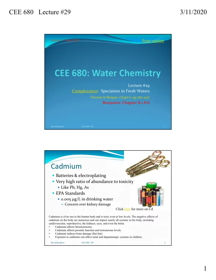
Cadmium
David Reckhow CEE 680 #29 2
Cadmium is of no use to the human body and is toxic even at low levels. The negative effects of cadmium on the body are numerous and can impact nearly all systems in the body, including cardiovascular, reproductive, the kidneys, eyes, and even the brain.
- Cadmium affects blood pressure.
- Cadmium affects prostate function and testosterone levels.
- Cadmium induces bone damage (Itai-ltai).
- Exposure to cadmium can affect renal and dopaminergic systems in children.
Batteries & electroplating Very high ratio of abundance to toxicity
Like Pb, Hg, As
EPA Standards
0.005 g/L in drinking water
Concern over kidney damage
Click here for more on Cd