SLIDE 12 Thresholds are in a logit scale:
The LCA model with p observed binary items u, has a categorical latent variable C with K classes (C = k; k = 1, 2, ..., K). The marginal item probability for item uj = 1 (j = 1, 2, ..., p) is given by: P (uj = 1) = sum P(C=k) * P (uj = 1 | C = k) where the conditional item probability in a given class is defined by : P (uj = j| C = k) = 1 / [ 1 + exp(- vjk) ] where the vjk is the logit for each of the ujs for each of the latent classes, k For example, if we want to constrain P(a=1|c=1) = .05, we fix logit threshold v(jk) to -2.95 [a$1@-2.95] ; A threshold = 0 will make P(a=1|c=1) = .50 ...and so on
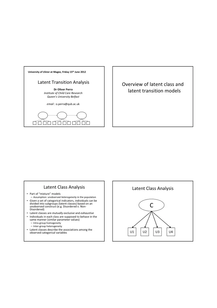
Intro to Mplus (ctd.)
MODEL: %OVERALL% !this is the part of the model common for all !classes [x#1]; %x#1% [a$1-d$1] (1-4); %x#2% [a$1-d$1] (5-8);
The parentheses after the indicators’ thresholds assign a name (if a letter is used) or posit a constraint (if a number used) to each of these parameters. If we wanted the thresholds of a, b, c and d to be the same for x1 and x2, we would have written: %x#1% [a$1-d$1] (1-4); %x#2% [a$1-d$1] (1-4); By doing this, we are making the thresholds, therefore the item response probabilities, the same for x=1 and x=2
This means that the threshold for the latent categorical variable is being estimated: where do you cut the latent variable distribution to form two latent classes, as specified by CLASSES = x(2); estimates prob of being in x1 class
Constraints on measurement model: Parallel indicators
MODEL: %OVERALL% !this is the part of the model common for all !classes
[x#1]; %x#1% [a$1-d$1] (1); %x#2% [a$1-d$1] (2); In this example, the thresholds for the latent class estimators (a to d: a, b, c, d) are equal to each other within each class, but not equal across classes given membership in class 1, the probability of endorsing indicator a is the same as the probability of endorsing item b, and so on. Referred as parallel indicators : have identical error rates with respect to each
- f the latent classes (if we consider one
type of response within class as an error)
MODEL: %OVERALL% [x#1]; %x#1% [a$1-b$1*-1] (1);
[c$1*-1] (p1);
[d$1*-1]; %x#2% [a$1-b$1*1] (2);
[c$1*1] (p2);
[d$1*1];
MODEL CONSTRAINT: p2 = - p1;
The * followed by a number assigns starting values to the thresholds, which helps specify the class meaning. In the example, class 1 is the class with negative starting values for thresholds, hence the class with higher probability of endorsing items (category 2 = endorsement). Thresholds for c are given names (p1, p2). A MODEL CONSTRAINT command defines a linear constraint: the threshold of c in class 1 is equal to the negative value of threshold of c in class 2. This effectively means that the probability of NOT endorsing item c in class 1 (the endorsers) is the same as the probability of endorsing item c in class 2 (the non-endorsers): Called equal error hypothesis: an indicator has the same error rate across the two classes (non
endorsement of an item in the endorsers class = a response error)