SLIDE 1
BORDERED FLOER HOMOLOGY HOMEWORK 2
ROBERT LIPSHITZ
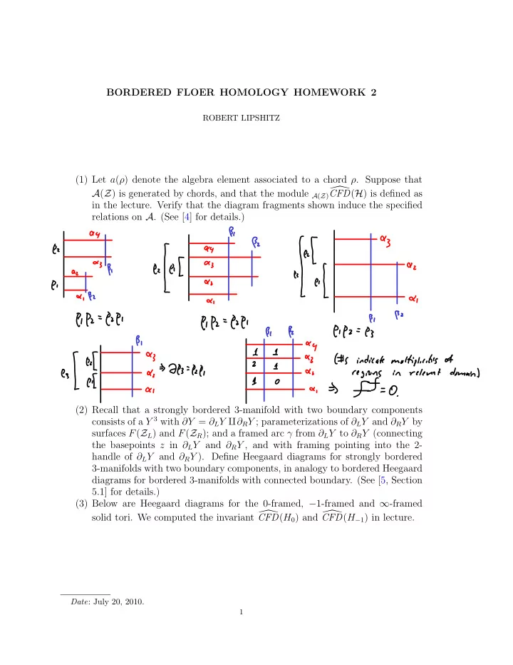
(1) Let a(ρ) denote the algebra element associated to a chord ρ. Suppose that A(Z) is generated by chords, and that the module A(Z) CFD(H) is defined as in the lecture. Verify that the diagram fragments shown induce the specified relations on A. (See [4] for details.) (2) Recall that a strongly bordered 3-manifold with two boundary components consists of a Y 3 with ∂Y = ∂LY ∐∂RY ; parameterizations of ∂LY and ∂RY by surfaces F(ZL) and F(ZR); and a framed arc γ from ∂LY to ∂RY (connecting the basepoints z in ∂LY and ∂RY , and with framing pointing into the 2- handle of ∂LY and ∂RY ). Define Heegaard diagrams for strongly bordered 3-manifolds with two boundary components, in analogy to bordered Heegaard diagrams for bordered 3-manifolds with connected boundary. (See [5, Section 5.1] for details.) (3) Below are Heegaard diagrams for the 0-framed, −1-framed and ∞-framed solid tori. We computed the invariant CFD(H0) and CFD(H−1) in lecture.
Date: July 20, 2010.
1
SLIDE 2 2 ROBERT LIPSHITZ
(a) Compute CFD(H∞). (b) Write down an exact sequence 0 → CFD(H∞) → CFD(H−1) → CFD(H0) → 0. What does this imply about HF(Y )? (4) This exercise relates to a diagram from [1] which can be used to show that
= ExtA(−F)( CFD(Y1), CFD(Y2)) ∼ = ExtA(F)( CFA(Y1), CFA(Y2)). (See [1] or [2].) For notational convenience, we will work in the genus 1 case. Let AZ denote the following strongly bordered Heegaard diagram: (Unlike the diagrams we will use in lecture, this one has α-arcs meeting one boundary component and β-arcs meeting the other.) (a) Prove (by direct computation) that CFAA(AZ) is isomorphic to A(T 2), as an A(T 2)-bimodule. (Hint: AZ is a nice diagram; see [3, Section 8], particularly Proposition 8.4.) (b) Aside: Use the pairing theorem and the previous part to show that if IZ denotes the identity Heegaard diagram for Z then CFDA(I) ≃ A as an A-bimodule. (c) Given a Heegaard diagram H, let H be the orientation-reverse of H. Prove that CFD(H) = CFD(H)∗, the dual of CFD(H). (d) Suppose H is a bordered Heegaard diagram for a 3-manifold Y with connected boundary. Let Hβ denote the result of relabeling the α-curves in H as β-curves and the β-curves as α-curves. Show that Hβ ∪∂ AZ is a bordered Heegaard diagram for −Y .
SLIDE 3
BORDERED FLOER HOMOLOGY HOMEWORK 2 3
(e) Challenge: Let H denote the result of gluing two copies of AZ along the boundary component intersecting the β-arcs (so H is an α-α-bordered Heegaard diagram.) What strongly bordered 3-manifold does H repre- sent? References
[1] Denis Auroux, Fukaya categories of symmetric products and bordered Heegaard-Floer homology, 2010, arXiv:1001.4323. [2] Robert Lipshitz, Peter S. Ozsv´ ath, and Dylan P. Thurston, Heegaard Floer homology as morphism spaces, in preparation. [3] , Bordered Heegaard Floer homology: Invariance and pairing, 2008, arXiv:0810.0687. [4] , Slicing planar grid diagrams: A gentle introduction to bordered Heegaard Floer homology, 2008, arXiv:0810.0695. [5] , Bimodules in bordered Heegaard Floer homology, 2010, arXiv:1003.0598. Department of Mathematics, Columbia University, New York, NY 10027 E-mail address: lipshitz@math.columbia.edu