Bookkeeping HW 1 due last night Grades within 1.5 weeks (hopefully - PowerPoint PPT Presentation

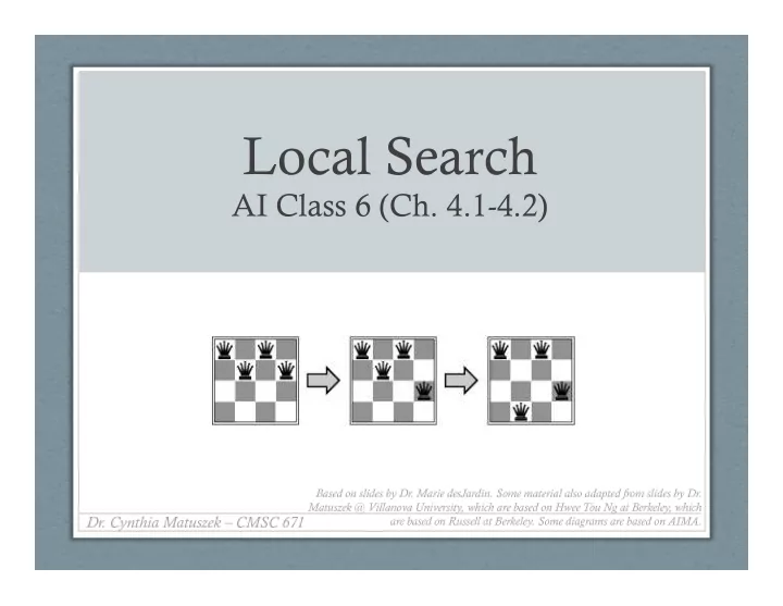
Local Search AI Class 6 (Ch. 4.1-4.2) Based on slides by Dr. Marie desJardin. Some material also adapted from slides by Dr. Matuszek @ Villanova University, which are based on Hwee Tou Ng at Berkeley, which Dr. Cynthia Matuszek – CMSC 671 are based on Russell at Berkeley. Some diagrams are based on AIMA.

Bookkeeping • HW 1 due last night • Grades within 1.5 weeks (hopefully sooner) • Discussions after grading • HW 2 out tonight 11:59 • Due 10/3, 11:59pm 2

Today’s Class • Iterative improvement methods • Hill climbing “If the path to the goal • Simulated annealing does not matter… [we can use] a single current • Local beam search node and move to • Genetic algorithms neighbors of that node.” – R&N pg. 121 • Online search 3

Admissibility • Admissibility is a property of heuristics • They are optimistic – think goal is closer than it is • (Or, exactly right) • Admissible algorithms can be pretty bad! • Is h ( n ): “1 kilometer” admissible? • Using admissible heuristics guarantees that the first solution found will be optimal, for some algorithms (A*). 4

Admissibility and Optimality • Intuitively: • When A* finds a path of length k , it has already tried every other path which can have length ≤ k • Because all frontier nodes have been sorted in ascending order of f ( n )= g ( n )+ h ( n ) • Does an admissible heuristic guarantee optimality for greedy search? • Reminder: f ( n ) = h ( n ), always choose node “nearest” goal • No sorting beyond that 5

Local Search Algorithms • Sometimes the path to the goal is irrelevant • Goal state itself is the solution E • an objective function to evaluate states • In such cases, we can use local search algorithms • Keep a single “current” state, try to improve it X 6

Local Search Algorithms Very efficient! • Sometimes the path to the goal is irrelevant • Goal state itself is the solution Why? • an objective function to evaluate states E • State space = set of “complete” configurations • That is, all elements of a solution are present • Find configuration satisfying constraints • Example? • In such cases, we can use local search algorithms • Keep a single “current” state, try to improve it 7

What Is This? 8

Iterative Improvement Search • Start with an initial guess • Gradually improve it until it is legal or optimal • Some examples: • Hill climbing • Simulated annealing • Constraint satisfaction 9

Hill Climbing on State Surface • Concept: trying to reach the “highest” (most desirable) point (state) • “Height” Defined by Evaluation Function 10

Hill Climbing Search • If there exists a successor s for the current state n such that • h ( s ) < h ( n ) • h ( s ) ≤ h ( t ) for all the successors t of n , then move from n to s . Otherwise, halt at n . • Look one step ahead to determine if any successor is “better” than current state • If so, move to the best successor • A kind of Greedy search in that it uses h • But, does not allow backtracking or jumping to an alternative path • Doesn’t “remember” where it has been. • Not complete • Search will terminate at local minima, plateaux, ridges. 11

Hill Climbing Example 2 8 3 2 1 3 start 1 6 4 8 4 h = 0 goal h = -4 7 5 7 6 5 -2 -5 -5 2 8 3 2 1 3 h = -3 1 4 8 4 h = -1 7 6 5 7 6 5 -3 -4 2 2 3 3 h = -2 1 8 4 1 8 4 7 6 5 7 6 5 h = -3 -4 f(n) = -(number of tiles out of place) 12

Exploring the Landscape local maximum • Local Maxima : • Peaks that aren’t the highest point in the space plateau • Plateaus: • A broad flat region that gives the search algorithm no direction (random walk) • Ridges: • Flat like a plateau, but with drop-offs to the sides; steps ridge to the North, East, South and West may go down, but a step to the NW may go up. Image from: http://classes.yale.edu/fractals/CA/GA/Fitness/Fitness.html

Drawbacks of Hill Climbing • Problems: local maxima, plateaus, ridges • Remedies: • Random restart: keep restarting the search from random locations until a goal is found. • Problem reformulation: reformulate the search space to eliminate these problematic features • Some problem spaces are great for hill climbing; others are terrible 14

Example of a Local Optimum 1 2 5 f = -7 7 4 move start goal up 8 6 3 1 2 5 1 2 3 8 7 4 8 4 f = 0 move 6 3 7 6 5 right 1 2 5 f = -6 f = -7 8 7 4 6 3 f = -(manhattan distance) 15

Some Extensions of Hill Climbing • Simulated Annealing • Escape local maxima by allowing some “bad” moves but gradually decreasing their frequency • Local Beam Search • Keep track of k states rather than just one • At each iteration: • All successors of the k states are generated and evaluated • Best k are chosen for the next iteration 16

Some Extensions of Hill Climbing • Stochastic Beam Search • Chooses semi-randomly from “uphill” possibilities • “Steeper” moves have a higher probability of being chosen • Random-Restart Climbing • Can actually be applied to any form of search • Pick random starting points until one leads to a solution • Genetic Algorithms • Each successor is generated from two predecessor (parent) states 17

Gradient Ascent / Descent • Gradient descent procedure for finding the arg x min f(x) • choose initial x 0 randomly • repeat • x i+1 ← x i – η f’ (x i ) • until the sequence x 0 , x 1 , …, x i , x i+1 converges • Step size η (eta) is small (~0.1–0.05) • Good for differentiable, continuous spaces 18 Images from http://en.wikipedia.org/wiki/Gradient_descent

Gradient Methods vs. Newton’s Method • A reminder of Newton’s method from Calculus: x i+1 ← x i – η f’ (x i ) / f’’ (x i ) • Newton ’ s method uses 2 nd order information (the second derivative, or, curvature ) to take a more direct route to the minimum. Contour lines of a function • The second-order information Gradient descent (green) is more expensive to compute, but converges more quickly. Newton’s method (red) Images from http://en.wikipedia.org/wiki/Newton's_method_in_optimization

Simulated Annealing • Simulated annealing (SA): analogy between the way metal cools into a minimum-energy crystalline structure and the search for a minimum generally • In very hot metal, molecules can move fairly freely • But, they are slightly less likely to move out of a stable structure • As you slowly cool the metal, more molecules are “trapped” in place • Conceptually: Escape local maxima by allowing some “bad” (locally counterproductive) moves but gradually decreasing their frequency 20

Simulated Annealing (II) • Can avoid becoming trapped at local minima. • Uses a random local search that: • Accepts changes that increase objective function f • As well as some that decrease it • Uses a control parameter T • By analogy with the original application • Is known as the system “ temperature ” • T starts out high and gradually decreases toward 0 21

Simulated Annealing (IIII) • f ( s ) represents the quality of state n (high is good) • A “bad” move from A to B is accepted with a probability P(move A → B ) ≈ e ( f (B) – f (A)) / T • (Note that f (B) – f (A) will be negative, so bad moves always have a relatively probability less than one. Good moves, for which f (B) – f (A) is positive, have a relative probability greater than one.) • Temperature • The higher the temperature, the more likely it is that a “bad” move can be made. • As T tends to zero, this probability tends to zero, and SA becomes more like hill climbing • If T is lowered slowly enough, SA is complete and admissible. 22

Visualizing SA Probabilities 2.5" 2" p(neg) = 1.5" 0.1422741 T=1" 1" 0.5" 0" (1.5" (1" (0.5" 0" 0.5" 1" 1.5" T=0.5$ [-1,1] ratio = 49.402449 8" 7" 6" p(neg) = 5" 0.0202419 4" T=0.5" 3" 2" 1" 0" T=0.1$ (1.5" (1" (0.5" 0" 0.5" 1" 1.5" 15000" [-1,1] ratio = 10000" 294267566 T=0.1" 5000" p(neg) = 23

The Simulated Annealing Algorithm 24

Local Beam Search • Begin with k random states • k , instead of one, current state(s) • Generate all successors of these states • Keep the k best states • Stochastic beam search • Probability of keeping a state is a function of its heuristic value • More likely to keep “better” successors 25

Genetic Algorithms • The Idea: • New states are generated by “mutating” a single state or “reproducing” (somehow combining) two parent states • Selected according to their fitness • Similar to stochastic beam search • Start with k random states (the initial population ) • Encoding used for the “genome” of an individual strongly affects the behavior of the search • Genetic algorithms / genetic programming are a large and active area of research 26

Class Exercise: Local Search for N-Queens Q Q Q Q Q Q 27 (more on constraint satisfaction heuristics next time...)