Dynamic Programming II Sequence alignment Shortest paths with - - PowerPoint PPT Presentation

Dynamic Programming II

Inge Li Gørtz KT section 6.6 and 6.8

Thank you to Kevin Wayne for inspiration to slides

1

• Optimal substructure
• Last time
• Weighted interval scheduling
• Segmented least squares
• Today
• Sequence alignment
• Shortest paths with negative weights

Dynamic Programming

2

Sequence Alignment

3

A C A A G T C

• C A T G T -
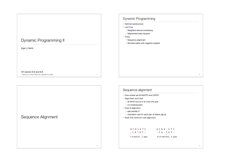
• How similar are ACAAGTC and CATGT.
• Align them such that
• all items occurs in at most one pair.
• no crossing pairs.
• Cost of alignment
• gap penalty δ
• mismatch cost for each pair of letters α(p,q).
• Goal: find minimum cost alignment.

Sequence alignment

A C A A - G T C

• C A - T G T -

1 mismatch, 2 gaps 0 mismatches, 4 gaps

A C A A G T C

• C A T G T -

A C A A G T C

• C A T G T -

4

• Subproblem property.
• SA(Xi,Yj) = min cost of aligning strings X[1…i] and Y[1…j].
• Case 1. Align xi and yj.
• Pay mismatch cost for xi and yj + min cost of aligning Xi-1 and Yj-1.
• Case 2. Leave xi unaligned.
• Pay gap cost + min cost of aligning Xi-1 and Yj.
• Case 3. Leave yj unaligned.
• Pay gap cost + min cost of aligning Xi and Yj-1.

Sequence Alignment

xi Xi-1 yj Yj-1

5

Sequence alignment

A C A A G T C C A T G T A C G T A 1 2 2 C 1 2 3 G 2 2 1 T 2 3 1 Penalty matrix SA(Xi, Yj) =                jδ if i = 0 iδ if j = 0 min      α(xi, yj) + SA(Xi−1, Yj−1), δ + SA(Xi, Yj−1), δ + SA(Xi−1, Yj)}

• therwise

δ = 1 SA(X5, Y3)

6

Sequence alignment

A C A A G T C C A T G T A C G T A 1 2 2 C 1 2 3 G 2 2 1 T 2 3 1 Penalty matrix SA(Xi, Yj) =                jδ if i = 0 iδ if j = 0 min      α(xi, yj) + SA(Xi−1, Yj−1), δ + SA(Xi, Yj−1), δ + SA(Xi−1, Yj)}

• therwise

δ = 1 SA(X5, Y3) Depends on ?

7

Sequence alignment

A C A A G T C C A T G T A C G T A 1 2 2 C 1 2 3 G 2 2 1 T 2 3 1 Penalty matrix SA(Xi, Yj) =                jδ if i = 0 iδ if j = 0 min      α(xi, yj) + SA(Xi−1, Yj−1), δ + SA(Xi, Yj−1), δ + SA(Xi−1, Yj)}

• therwise

δ = 1 SA(X5, Y3) Depends on ?

8

Sequence alignment

A C A A G T C 1 2 3 4 5 6 7 C 1 A 2 T 3 G 4 T 5 A C G T A 1 2 2 C 1 2 3 G 2 2 1 T 2 3 1 Penalty matrix SA(Xi, Yj) =                jδ if i = 0 iδ if j = 0 min      α(xi, yj) + SA(Xi−1, Yj−1), δ + SA(Xi, Yj−1), δ + SA(Xi−1, Yj)}

• therwise

δ = 1

9

Sequence alignment

A C A A G T C 1 2 3 4 5 6 7 C 1 A 2 T 3 G 4 T 5 A C G T A 1 2 2 C 1 2 3 G 2 2 1 T 2 3 1 Penalty matrix SA(Xi, Yj) =                jδ if i = 0 iδ if j = 0 min      α(xi, yj) + SA(Xi−1, Yj−1), δ + SA(Xi, Yj−1), δ + SA(Xi−1, Yj)}

• therwise

δ = 1 min( ) 1+0, 1+1, 1+1

10

Sequence alignment

A C A A G T C 1 2 3 4 5 6 7 C 1 1 A 2 T 3 G 4 T 5 A C G T A 1 2 2 C 1 2 3 G 2 2 1 T 2 3 1 Penalty matrix SA(Xi, Yj) =                jδ if i = 0 iδ if j = 0 min      α(xi, yj) + SA(Xi−1, Yj−1), δ + SA(Xi, Yj−1), δ + SA(Xi−1, Yj)}

• therwise

δ = 1 min( ) 1+0, 1+1, 1+1

11

Sequence alignment

A C A A G T C 1 2 3 4 5 6 7 C 1 1 A 2 T 3 G 4 T 5 A C G T A 1 2 2 C 1 2 3 G 2 2 1 T 2 3 1 Penalty matrix SA(Xi, Yj) =                jδ if i = 0 iδ if j = 0 min      α(xi, yj) + SA(Xi−1, Yj−1), δ + SA(Xi, Yj−1), δ + SA(Xi−1, Yj)}

• therwise

δ = 1 min( ) 0+1, 1+2, 1+1

12

Sequence alignment

A C A A G T C 1 2 3 4 5 6 7 C 1 1 1 A 2 T 3 G 4 T 5 A C G T A 1 2 2 C 1 2 3 G 2 2 1 T 2 3 1 Penalty matrix SA(Xi, Yj) =                jδ if i = 0 iδ if j = 0 min      α(xi, yj) + SA(Xi−1, Yj−1), δ + SA(Xi, Yj−1), δ + SA(Xi−1, Yj)}

• therwise

δ = 1 min( ) 0+1, 1+2, 1+1

13

Sequence alignment

A C A A G T C 1 2 3 4 5 6 7 C 1 1 1 A 2 T 3 G 4 T 5 A C G T A 1 2 2 C 1 2 3 G 2 2 1 T 2 3 1 Penalty matrix SA(Xi, Yj) =                jδ if i = 0 iδ if j = 0 min      α(xi, yj) + SA(Xi−1, Yj−1), δ + SA(Xi, Yj−1), δ + SA(Xi−1, Yj)}

• therwise

δ = 1 min(1+2, 1+3, 1+1)

14

Sequence alignment

A C A A G T C 1 2 3 4 5 6 7 C 1 1 1 2 A 2 T 3 G 4 T 5 A C G T A 1 2 2 C 1 2 3 G 2 2 1 T 2 3 1 Penalty matrix SA(Xi, Yj) =                jδ if i = 0 iδ if j = 0 min      α(xi, yj) + SA(Xi−1, Yj−1), δ + SA(Xi, Yj−1), δ + SA(Xi−1, Yj)}

• therwise

δ = 1 min(1+2, 1+3, 1+1)

15

Sequence alignment

A C A A G T C 1 2 3 4 5 6 7 C 1 1 1 2 A 2 T 3 G 4 T 5 A C G T A 1 2 2 C 1 2 3 G 2 2 1 T 2 3 1 Penalty matrix SA(Xi, Yj) =                jδ if i = 0 iδ if j = 0 min      α(xi, yj) + SA(Xi−1, Yj−1), δ + SA(Xi, Yj−1), δ + SA(Xi−1, Yj)}

• therwise

δ = 1 min(1+3, 1+4, 1+2)

16

Sequence alignment

A C A A G T C 1 2 3 4 5 6 7 C 1 1 1 2 3 A 2 T 3 G 4 T 5 A C G T A 1 2 2 C 1 2 3 G 2 2 1 T 2 3 1 Penalty matrix SA(Xi, Yj) =                jδ if i = 0 iδ if j = 0 min      α(xi, yj) + SA(Xi−1, Yj−1), δ + SA(Xi, Yj−1), δ + SA(Xi−1, Yj)}

• therwise

δ = 1 min(1+3, 1+4, 1+2)

17

Sequence alignment

A C A A G T C 1 2 3 4 5 6 7 C 1 1 1 2 3 4 A 2 T 3 G 4 T 5 A C G T A 1 2 2 C 1 2 3 G 2 2 1 T 2 3 1 Penalty matrix SA(Xi, Yj) =                jδ if i = 0 iδ if j = 0 min      α(xi, yj) + SA(Xi−1, Yj−1), δ + SA(Xi, Yj−1), δ + SA(Xi−1, Yj)}

• therwise

δ = 1 min(2+4, 1+5, 1+3)

18

Sequence alignment

A C A A G T C 1 2 3 4 5 6 7 C 1 1 1 2 3 4 5 6 A 2 1 2 1 2 3 4 5 T 3 2 3 2 3 3 3 4 G 4 3 4 3 4 3 4 5 T 5 4 5 4 5 4 3 4 A C G T A 1 2 2 C 1 2 3 G 2 2 1 T 2 3 1 Penalty matrix SA(Xi, Yj) =                jδ if i = 0 iδ if j = 0 min      α(xi, yj) + SA(Xi−1, Yj−1), δ + SA(Xi, Yj−1), δ + SA(Xi−1, Yj)}

• therwise

δ = 1

19

SA(X[1…m],Y[1…n],δ,A){ for i=0 to m M[i,0] := iδ for j=0 to n M[0,j] := jδ for i=1 to m for j = 1 to n M[i,j] := min{ A[i,j] + M[i-1,j-1], δ + M[i-1,j], δ + M[i,j-1]} Return M[m,n] }

Sequence alignment

20

• Time: Ɵ(mn)
• Space: Ɵ(mn)

Sequence alignment: Finding the solution

A C A A G T C 1 2 3 4 5 6 7 C 1 1 1 2 3 4 5 6 A 2 1 2 1 2 3 4 5 T 3 2 3 2 3 3 3 4 G 4 3 4 3 4 3 4 5 T 5 4 5 4 5 4 3 4 A C G T A 1 2 2 C 1 2 3 G 2 2 1 T 2 3 1 Penalty matrix

SA(Xi, Yj) =                jδ if i = 0 iδ if j = 0 min      α(xi, yj) + SA(Xi−1, Yj−1), δ + SA(Xi, Yj−1), δ + SA(Xi−1, Yj)}

• therwise

δ = 1 A C A A G T C

← ← ← ← ← ← ←

C ↑

↖ ↖ ← ← ← ← ↖

A

↑ ↖ ↖ ↖ ↖ ← ← ←

T ↑

↑ ↑ ↑ ↖ ↖ ↖ ←

G ↑

↑ ↖ ↑ ↖ ↖ ↖ ↖

T ↑

↑ ↑ ↑ ↖ ↑ ↖ ←

21

• Use dynamic programming to compute an optimal alignment.
• Time: Ɵ(mn)
• Space: Ɵ(mn)
• Find actual alignment by backtracking (or saving information in another matrix).
• Linear space?
• Easy to compute value (save last and current row)
• How to compute alignment? Hirschberg. (not part of the curriculum).

Sequence alignment

22

Shortest paths

23

• All-Pairs Shortest Path Problem (APSP)
• Given directed weighted graph G=(V,E).
• Weights of edges cij are real numbers (might be negative).
• Let n = |V| and m= |E|.
• Weight of a path is the sum of the weights on its edges.
• Goal: Compute the shortest path for from node s to node t.

Shortest Paths

s t 9 10 6 18 15

• 8

30 20 44

• 16

11 6 19 6 16

24

• All-Pairs Shortest Path Problem (APSP)
• Given directed weighted graph G=(V,E).
• Weights of edges cij are real numbers (might be negative).
• Let n = |V| and m= |E|.
• Weight of a path is the sum of the weights on its edges.
• Goal: Compute the shortest path for from node s to node t.

Shortest Paths

s t 9 10 6 18 15

• 8

30 20 44

• 16

11 6 19 6 16

25

• All-Pairs Shortest Path Problem (APSP)
• Given directed weighted graph G=(V,E).
• Weights of edges cij are real numbers (might be negative).
• Let n = |V| and m= |E|.
• Weight of a path is the sum of the weights on its edges.
• Goal: Compute the shortest path for from node s to node t.

Shortest Paths

s t 9 10 6 18 15

• 8

30 20 44

• 16

11 6 19 6 16

• 26
• Dijkstra
• Re-weighting

Failed attempts

s t 3 2

• 3

3 2 5 5 6 6

27

s 2 1

• 10

2 t 1

• Negative cycle. If some path from s to t contains a negative cost cycle, then there

does not exist a shortest s-t path. Otherwise, there exists one that is simple.

• Optimal substructure. Subpaths of shortest paths are shortest paths

Observations

s t

28

• OPT(i,v) = length of shortest v-t path P using at most i edges.
• Case 1: P uses at most i-1 edges.
• Case 2: P uses exactly i edges.
• If no negative cycles then OPT(n-1,v) = length of shortest path

Recurrence

t v

w

shortest w ➝ t path using at most i-1 edges cvw v

t

shortest v ➝ t path using at most i-1 edges

OPT(i,v) = OPT(i-1,v) OPT(i,v) = OPT(i-1,w) + cvw

OPT(i, v) = { if i = 0 min{OPT(i − 1,v), min(v,w)∈E{OPT(i − 1,w) + cvw}}

• therwise

29

Bellman-Ford

OPT(i, v) = { if i = 0 min{OPT(i − 1,v), min(v,w)∈E{OPT(i − 1,w) + cvw}}

• therwise

Bellmann-Ford(G,s,t) for each node v ∈ V M[0,v] = ∞ M[0,t] = 0. for i=1 to n-1 for each node v ∈ V M[i,v] = M[i-1,v] for each edge (v,w) ∈ E M[i,v] = min(M[i,v], M[i-1,w] + cvw)

30

Example

s t 9 10 6 18 15

• 8

30 20 44

• 16

11 6 19 6 16 ∞ ∞ ∞ ∞ ∞ ∞ ∞

Bellmann-Ford(G,s,t) for each node v ∈ V M[0,v] = ∞ M[0,t] = 0. for i=1 to n-1 for each node v ∈ V M[i,v] = M[i-1,v] for each edge (v,w) ∈ E M[i,v] = min(M[i,v], M[i-1,w] + cvw

31

1 2 3 4 5 6 7 s ∞ a ∞ b ∞ c ∞ d ∞ e ∞ f ∞ t

a d b e c f

Example

s t 9 10 6 18 15

• 8

30 20 44

• 16

11 6 19 6 16

32

a d b e c f

1 2 3 4 5 6 7 s ∞ a ∞ b ∞ c ∞ d ∞ e ∞ f ∞ t ∞ ∞ ∞ 44 16 6 19

∞ ∞ ∞ ∞ ∞ ∞ ∞ 6 16 44 19

Bellmann-Ford(G,s,t) for each node v ∈ V M[0,v] = ∞ M[0,t] = 0. for i=1 to n-1 for each node v ∈ V M[i,v] = M[i-1,v] for each edge (v,w) ∈ E M[i,v] = min(M[i,v], M[i-1,w] + cvw

Example

s t 9 10 6 18 15

• 8

30 20 44

• 16

11 6 19 6 16 ∞ ∞ ∞ 19 6 44 16 59 29 36

33

a d b e c f

1 2 3 4 5 6 7 s ∞ ∞ a ∞ ∞ b ∞ ∞ c ∞ 44 d ∞ 16 e ∞ 6 f ∞ 19 t 59 29 36 44 16 6 Bellmann-Ford(G,s,t) for each node v ∈ V M[0,v] = ∞ M[0,t] = 0. for i=1 to n-1 for each node v ∈ V M[i,v] = M[i-1,v] for each edge (v,w) ∈ E M[i,v] = min(M[i,v], M[i-1,w] + cvw

Example

s t 9 10 6 18 15

• 8

30 20 44

• 16

11 6 19 6 16 36 29 59 6 44 16 38 10 18

34

a d b e c f

1 2 3 4 5 6 7 s ∞ ∞ 59 a ∞ ∞ 29 b ∞ ∞ 36 c ∞ 44 44 d ∞ 16 16 e ∞ 6 6 f ∞ 19 t 38 10 18 44 16 6 Bellmann-Ford(G,s,t) for each node v ∈ V M[0,v] = ∞ M[0,t] = 0. for i=1 to n-1 for each node v ∈ V M[i,v] = M[i-1,v] for each edge (v,w) ∈ E M[i,v] = min(M[i,v], M[i-1,w] + cvw

Example

s t 9 10 6 18 15

• 8

30 20 44

• 16

11 6 19 6 16 18 10 38 6 44 16 19

35

a d b e c f

1 2 3 4 5 6 7 s ∞ ∞ 59 38 a ∞ ∞ 29 10 b ∞ ∞ 36 18 c ∞ 44 44 44 d ∞ 16 16 16 e ∞ 6 6 6 f ∞ 19 t 19 10 18 44 16 6 Bellmann-Ford(G,s,t) for each node v ∈ V M[0,v] = ∞ M[0,t] = 0. for i=1 to n-1 for each node v ∈ V M[i,v] = M[i-1,v] for each edge (v,w) ∈ E M[i,v] = min(M[i,v], M[i-1,w] + cvw

Example

s t 9 10 6 18 15

• 8

30 20 44

• 16

11 6 19 6 16 18 10 19 6 44 16

36

a d b e c f

1 2 3 4 5 6 7 s ∞ ∞ 59 38 19 a ∞ ∞ 29 10 10 b ∞ ∞ 36 18 18 c ∞ 44 44 44 44 d ∞ 16 16 16 16 e ∞ 6 6 6 6 f ∞ 19 t 19 10 18 44 16 6 Bellmann-Ford(G,s,t) for each node v ∈ V M[0,v] = ∞ M[0,t] = 0. for i=1 to n-1 for each node v ∈ V M[i,v] = M[i-1,v] for each edge (v,w) ∈ E M[i,v] = min(M[i,v], M[i-1,w] + cvw

Example

s t 9 10 6 18 15

• 8

30 20 44

• 16

11 6 19 6 16 18 10 19 6 44 16

37

a d b e c f

1 2 3 4 5 6 7 s ∞ ∞ 59 38 19 19 19 19 a ∞ ∞ 29 10 10 10 10 10 b ∞ ∞ 36 18 18 18 18 18 c ∞ 44 44 44 44 44 44 44 d ∞ 16 16 16 16 16 16 16 e ∞ 6 6 6 6 6 6 6 f ∞ 19 t

can stop when no changes in a round

Bellmann-Ford(G,s,t) for each node v ∈ V M[0,v] = ∞ M[0,t] = 0. for i=1 to n-1 for each node v ∈ V M[i,v] = M[i-1,v] for each edge (v,w) ∈ E M[i,v] = min(M[i,v], M[i-1,w] + cvw

Bellman-Ford

Bellmann-Ford(G,s,t) for each node v ∈ V M[v] = ∞ M[t] = 0. for i=1 to n-1 for each node v ∈ V M[i,v] = M[i-1,v] for each edge (v,w) ∈ E M[i,v] = min(M[i,v], M[i-1,w] + cvw

• Running time. O(mn)
• Space. O(n2)

38

• Improvements to basic implementation
• Maintain only one array
• No need to check edges of form (v,w) if M[w] didn’t change in previous iteration.
• Space: O(m+n)
• Running time: O(mn) worst case, but substantially faster in practice.

Bellman-Ford

Bellmann-Ford-push-based(G,s,t) for each node v ∈ V M[v] = ∞ succ[v] = nil M[t] = 0. for i=1 to n-1 for each node w ∈ V if M[w] was updated in previous iteration do for each node v such that (v,w) ∈ E if M[v] > M[w] + cvw do

M[v] = M[w] + cvw

succ[v] = w if no M[w] changed in iteration i, stop.

39

• Lemma. If OPT(n,v) < OPT(n-1,v) for some node, then (any) shortest path from v to t

contains a cycle C with negative cost.

• Proof. By contradiction.
• OPT(n,v) < OPT(n-1,v) => P has exactly n edges
• => P contains a cycle C.
• Deleting C gives a v-t path with < n edges => C makes v-t path shorter => C has

negative cost.

• Lemma. If OPT(n,v) = OPT(n-1,v) for all v, then no negative cycles.

Detecting negative cycles

v t C

40

• Detect negative cost cycles in O(mn) time.
• Add new node t and connect all nodes to t with 0-cost edge.
• Check if OPT(n,v) = OPT(n-1,v) for all nodes v.
• Yes: No negative cycles.
• No: Can find negative cycle from shortest path from v to t.

Detecting negative cycles

t 18

• 8

30 20

• 16

11 6

• 41