Binocular Stereo Take 2 images from different known viewpoints 1 - PDF document

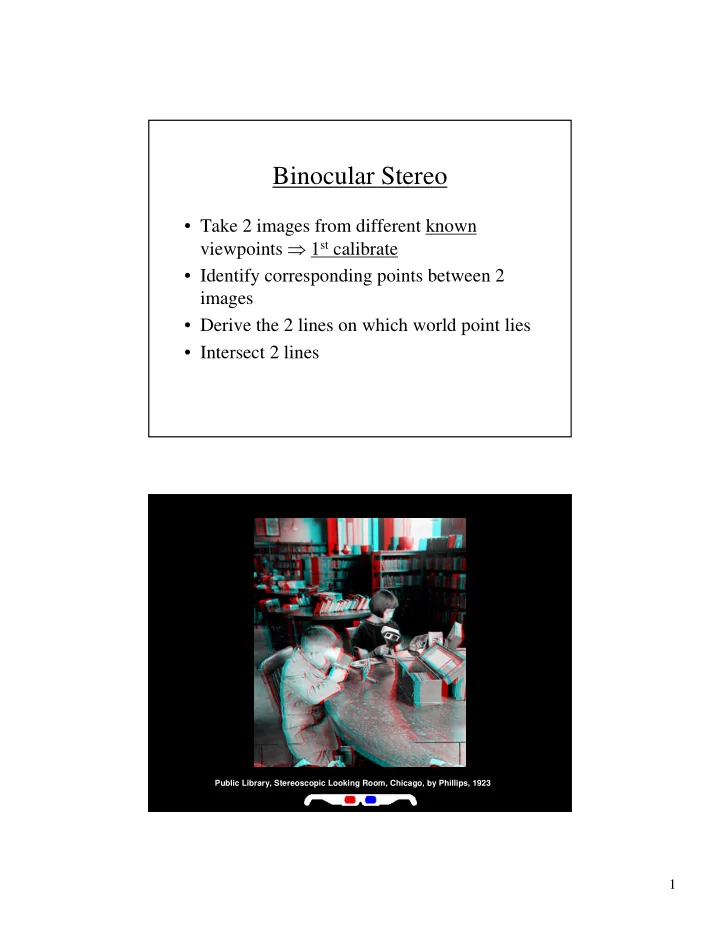
Binocular Stereo • Take 2 images from different known viewpoints ⇒ 1 st calibrate • Identify corresponding points between 2 images • Derive the 2 lines on which world point lies • Intersect 2 lines Public Library, Stereoscopic Looking Room, Chicago, by Phillips, 1923 1

2

Stereo • Basic Principle: Triangulation – Gives reconstruction as intersection of two rays – Requires • calibration • point correspondence 3

Depth from Disparity input image (1 of 2) depth map 3D rendering [Szeliski & Kang ‘95] X z u u’ f f baseline C C’ 4

Multi-View Geometry • Different views of a scene are not unrelated • Several relationships exist between two, three and more cameras • Question: Given an image point in one image, does this restrict the position of the corresponding image point in another image? 5

Epipolar Geometry: Formalism • Depth can be reconstructed based on corresponding points (disparity) • Finding corresponding points is hard & computationally expensive • Epipolar geometry helps to significantly reduce search from 2-D to 1-D line Epipolar Geometry: Demo Java Applet http://www- sop.inria.fr/robotvis/personnel/sbougnou/Meta3DViewer/EpipolarGeo.html Sylvain Bougnoux, INRIA Sophia Antipolis 6

• Scene point P projects to image point p l = ( x l , y l , f l ) in left image and point p r = ( x r , y r , f r ) in right image • Epipolar plane contains P , O l , O r , p l and p r – called co-planarity constraint • Given point p l in left image, its corresponding point in right image is on line defined by intersection of epipolar plane defined by p l , O l , O r and image I r – called epipolar line of p l • In other words, p l and O l define a ray where P may lie; projection of this ray into I r is the epipolar line Marc Pollefeys, University of Leuven, Belgium, Siggraph 2001 Course 7

Epipolar Line Geometry • Epipolar Constraint : The correct match for a point p l is constrained to a 1D search along the epipolar line in I r • All epipolar planes defined by all points in I l contain the line O l O r ⇒ All epipolar lines in I r intersect at a point, e r , called the epipole • Left and right epipoles, e l and e r , defined by the intersection of line O l O r with the left and right images I l and I r , respectively 8

9

Epipolar Geometry Marc Pollefeys, University of Leuven, Belgium, Siggraph 2001 Course Epipolar Geometry: Rectification • [Trucco 157-160] • Motivation : Simplify search for corresponding points along scan lines (avoids interpolation and simplify sampling) • Technique : Image planes parallel -> pairs of conjugate epipolar lines become collinear and parallel to image axis. 10

Stereo Image Rectification • Image Reprojection – reproject image planes onto common plane parallel to line between optical centers – a homography (3x3 transform) applied to both input images – pixel motion is horizontal after this transformation – C. Loop and Z. Zhang, Computing Rectifying Homographies for Stereo Vision, Computer Vision and Pattern Recognition Conf., 1999 Rectification Marc Pollefeys, University of Leuven, Belgium, Siggraph 2001 Course 11

Rectification Example before after Rectification Procedure Given: Intrinsic and extrinsic parameters for 2 cameras 1. Rotate left camera so that the epipole goes to infinity along the horizontal axis ⇒ left image parallel to baseline 2. Rotate right camera using same transformation 3. Rotate right camera by R, the transformation of the right camera frame with respect to the left camera 4. Adjust scale in both cameras Implement as backward transformations, and resample using bilinear interpolation 12

Definitions • Conjugate Epipolar Line: A pair of epipolar lines in I l and I r defined by P , O l and O r • Conjugate (i.e., corresponding) Pair: A pair of matching image points from I l and I r that are projections of a single scene point 13

14

15

16

17

18

19

20

Basic Stereo Algorithm For each epipolar line For each pixel in the left image • compare with every pixel on same epipolar line in right image • pick pixel with minimum match cost Improvement: match windows 21

Stereo Correspondence disparities left image right image (x1,y) (x2,y) stereo disparity = x1 - x2 is inversely proportional to depth 3D scene structure recovery 22

Stereo Matching • Features vs. pixels? – Do we extract features prior to matching? Julesz-style Random Dot Stereogram 23

Difficulties in Stereo Correspondence left image right image Perfect case : never happens! 1) Image noise: 2) Low texture: ? ? 24

Local Approach • Look at one image patch at at time • Solve many small problems independently • Faster, less accurate Global Approach • Look at the whole image • Solve one large problem • Slower, more accurate How Difficult is Correspondence? high texture • local works for high texture • enough texture in a patch to disambiguate d i f f i c u l t y medium texture • global works up to medium texture • propagates estimates from textured to untextured regions • salient regions work up to low low texture texture • propagation fails; some regions are inherently ambiguous, match only unambiguous regions 25

Local Approach [Levine’73] left image right image 3 2 1 p C C C 3 2 1 d = i which gives best C p i 2 2 + + = Common C 2 2 + (SSD) Fixed Window Size Problems window shapes need different left image true disparities fixed small window fixed large window 26

Window Size W = 3 W = 20 • Effect of window size Better results with adaptive window – Smaller window • T. Kanade and M. Okutomi, A Stereo + Matching Algorithm with an Adaptive Window: Theory and Experiment , Proc. – Int. Conf. Robotics and Automation, – Larger window 1991 • D. Scharstein and R. Szeliski. Stereo + matching with nonlinear diffusion, Int. J. – Computer Vision, 28 (2):155-174, 1998 Sample Compact Windows [Veksler 2001] 27

Comparison to Fixed Window true disparities Veksler’s compact windows:16% errors fixed small window: 33% errors fixed large window: 30% errors Results (% Errors) Tsukuba Sawtooth Algorithm Venus Map Layered 1.58 1.52 0.34 0.37 Graph cuts 1.94 1.79 1.30 0.31 l a b Belief prop 1.15 1.00 0.98 0.84 o l g GC+occl. 1.27 2.79 0.36 1.79 l l a Graph cuts 1.86 1.69 0.42 2.39 Multiw. Cut 8.08 0.53 0.61 0.26 Veksler’s var. 3.36 1.67 1.61 0.33 windows 28

Constraints 1) corresponding pixels should be close in color q p 2) most nearby pixels should have similar disparity disparity except a few continuous places: in most disparity places discontinuity Additional geometric constraints for correspondence A B C • Ordering of points : Continuous surface: same order in both images. • Is that always true? A B C A B C A B C 29

Forbidden Zone N Practical applications: – Object bulges out: ok Forbidden M – In general: ordering Zone of M across whole image is not reliable feature – Use ordering constraints for neighbors of M within small neighborhood m 1 n 1 n 2 m 2 only 30

31

32

33

34

35

36

37

38

Global Approach [Horn’81, Poggio’84, …] encode desirable properties of d in E ( d ): d d d p q E ( d )= E r 2 MAP-MRF ∑ ∑ ( ( ) ) ( ) ( ( ) ) = + arg min E d M d P d , d p p q d { { } } ∈ ∈ Ρ ∈ Ν Ν p p , q eighbors match pixels of most nearby pixels similar color have similar disparity NP-hard problem ⇒ need approximations 39

Stereo as Energy Minimization • Matching cost formulated as energy – “data” term penalizing bad matches = − + ( , , ) I ( , ) J ( , ) D x y d x y x d y – “neighborhood term” encouraging spatial smoothness (continuity; disparity gradient) = V ( d , d ) cost of adjacent pixels with labels d1 and d2 1 2 = − d d (or something similar) 1 2 ∑ ∑ = + ( , , ) ( , ) E D x y d V d d x , y x 1 , y 1 x 2 , y 2 ( x , y ) neighbors ( x 1 , y 1 ), ( x 2 , y 2 ) Minimization Methods 1. Continuous d : Gradient Descent – Gets stuck in local minimum 2. Discrete d : Simulated Annealing [Geman and Geman, PAMI 1984] – Takes forever or gets stuck in local minimum 40

Stereo as a Graph Problem [Boykov, 1999] edge weight ( , , ) D x y d 3 d 3 d 2 d 1 edge weight Labels Pixels V ( d 1 d , ) 1 (disparities) Graph Definition d 3 d 2 d 1 • Initial state – Each pixel connected to it’s immediate neighbors – Each disparity label connected to all of the pixels 41