Belief Networks Some Belief Network references E. Charniak Bayesian - PowerPoint PPT Presentation

Belief Networks Some Belief Network references • E. Charniak “Bayesian Networks without Tears”, AI Magazine Winter 1991, pp 50-63 Chris Williams, School of Informatics University of Edinburgh • D. Heckerman, “A Tutorial on Learning Bayesian Networks”, Technical Report MSR-TR-95-06, Microsoft Research, March, 1995, • Independence http://research.microsoft.com/~heckerman/ • Conditional Independence • J. Pearl “Probabilistic Reasoning in Intelligent Systems: Networks of Plausible Inference”, Morgan Kaufmann, 1988 • Belief networks • R. E. Neapolitan “Probabilistic Reasoning in Expert Systems”, Wiley, 1990 • Constructing belief networks • E. Castillo, J. M. Guti´ errez, A. S. Hadi “Expert Systems and Probabilistic Network • Inference in belief networks Models”, Springer, 1997 • Learning in belief networks • S. J. Russell and P . Norvig, “Artificial Intelligence: A Modern Approach”, Prentice Hall, 1995 (chapters 14, 15) • Readings: e.g. Russell and Norvig, § 15.1, § 15.2, § 15.5, Jordan § 2.1 (details of Bayes ball algorithm optional) • F . V. 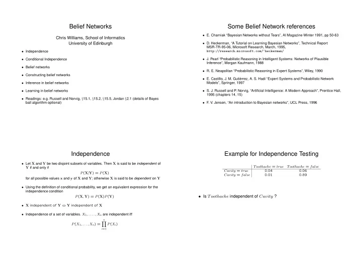Jensen, “An introduction to Bayesian networks”, UCL Press, 1996 Independence Example for Independence Testing • Let X and Y be two disjoint subsets of variables. Then X is said to be independent of Toothache = true Toothache = false Y if and only if Cavity = true 0 . 04 0 . 06 P ( X | Y ) = P ( X ) Cavity = false 0 . 01 0 . 89 for all possible values x and y of X and Y ; otherwise X is said to be dependent on Y • Using the definition of conditional probability, we get an equivalent expression for the independence condition • Is Toothache independent of Cavity ? P ( X , Y ) = P ( X ) P ( Y ) • X independent of Y ⇔ Y independent of X • Independence of a set of variables. X 1 , . . . . , X n are independent iff n � P ( X 1 , . . . , X n ) = P ( X i ) i =1

Conditional Independence Graphically Z Z • Let X , Y and Z be three disjoint sets of variables. X is said to be conditionally independent of Y given Z iff No independence, P ( X, Y, Z ) = Y Y P ( x | y , z ) = P ( x | z ) P ( Z ) P ( Y | Z ) P ( X | Y, Z ) for all possible values of x , y and z . I ( X , Y | Z ) ⇒ P ( X, Y, Z ) = X X P ( Z ) P ( Y | Z ) P ( X | Z ) • Equivalently P ( x , y | z ) = P ( x | z ) P ( y | z ) • Notation, I ( X , Y | Z ) Belief Networks Belief Networks 2 • A simple, graphical notation for conditional independence assertions and hence for • DAG ⇒ no directed cycles ⇒ can number nodes so that no edges go from a node to compact specification of full joint distributions another node with a lower number • Syntax: • Joint distribution n – a set of nodes, one per variable � P ( X 1 , . . . , X n ) = P ( X i | Parents ( X i )) – a directed acyclic graph (DAG) (link ≈ “directly influences”) i =1 – a conditional distribution for each node given its parents: P ( X i | Parents ( X i )) • Missing links imply conditional independence • In the simplest case, conditional distribution represented as a conditional probability • Ancestral simulation to sample from joint distribution table (CPT)

Example Belief Network • Unstructured joint distribution requires 2 5 − 1 = 31 numbers to specify it. Here can use 12 numbers P(f=empty) = 0.05 P(b=bad) = 0.02 Battery Fuel • Take the ordering b, f, g, t, s . Joint can be expressed as P ( b, f, g, t, s ) = P ( b ) P ( f | b ) P ( g | b, f ) P ( t | b, f, g ) P ( s | b, f, g, t ) Gauge P(g=empty|b=good, f=not empty) = 0.04 P(g=empty| b=good, f=empty) = 0.97 P(g=empty| b=bad, f=not empty) = 0.10 • Conditional independences (missing links) give P(g=empty|b=bad, f=empty) = 0.99 Turn Over P ( b, f, g, t, s ) = P ( b ) P ( f ) P ( g | b, f ) P ( t | b ) P ( s | t, f ) P(t=no|b=good) = 0.03 Start P(t=no|b=bad) = 0.98 P(s=no|t=yes, f=not empty) = 0.01 • What is probability of P(s=no|t=yes, f=empty) = 0.92 Heckerman (1995) P(s=no| t = no, f=not empty) = 1.0 P ( b = good, t = no, g = empty, f = not empty, s = no ) ? P(s=no| t = no, f = empty) = 1.0 Constructing belief networks • This procedure is guaranteed to produce a DAG 1. Choose a relevant set of variables X i that describe the domain • To ensure maximum sparsity, add “root causes” fi rst, then the variables they influence and so on, until leaves are reached. Leaves have no direct causal influence over other variables 2. Choose an ordering for the variables 3. While there are variables left • Example : Construct DAG for the car example using the ordering s, t, g, f, b (a) Pick a variable X i and add it to the network (b) Set Parents ( X i ) to some minimal set of nodes already in the net • “Wrong” ordering will give same joint distribution, but will require the specifi cation of more numbers than otherwise necessary (c) Defi ne the CPT for X i

Defi ning CPTs Conditional independence relations in belief networks • Where do the numbers come from? Can be elicted from experts, or • Consider three disjoint groups of nodes, X , Y , E learned see later • Q: Given a graphical model, how can we tell if I ( X , Y | E ) ? • CPTs can still be very large (and diffi cult to specify) if there are many parents for a node. Can use combination rules such as Pearl’s (1988) • A: we use a test called direction-dependent separation or d-separation NOISY-OR model for binary nodes • If every undirected path from X to Y is blocked by E , then I ( X , Y | E ) Defi ning blocked Example A A B B A B P(f=empty) = 0.05 P(b=bad) = 0.02 Battery Fuel C C C C is head-to-head C is tail-to-tail C is head-to-tail Gauge P(g=empty|b=good, f=not empty) = 0.04 P(g=empty| b=good, f=empty) = 0.97 P(g=empty| b=bad, f=not empty) = 0.10 A path is blocked if P(g=empty|b=bad, f=empty) = 0.99 Turn Over 1. there is a node ω ∈ E which is head-to-tail wrt the path P(t=no|b=good) = 0.03 P(t=no|b=bad) = 0.98 Start • I ( t, f |∅ ) ? 2. there is a node ω ∈ E which is tail-to-tail wrt the path P(s=no|t=yes, f=not empty) = 0.01 • I ( b, f | s ) ? P(s=no|t=yes, f=empty) = 0.92 Heckerman (1995) P(s=no| t = no, f=not empty) = 1.0 3. there is a node that is head-to-head and neither the node, nor any of its descendants, • I ( b, s | t ) ? P(s=no| t = no, f = empty) = 1.0 are in E

The Bayes Ball Algorithm Inference in belief networks • § 2.1 in Jordan (2003) • Inference is the computation of results to queries given a network in the presence of evidence • Paper “Bayes-Ball: The Rational Pastime” by R. D. Shachter (UAI 98) • e.g. All/specifi c marginal posteriors e.g. P ( b | s ) • Provides an algorithm with linear time complexity which given sets of nodes X and E , determines the set of nodes Y s.t. • e.g. Specifi c joint conditional queries e.g. P ( b, f | t ) , or fi nding the most likely explanation given the evidence I ( X , Y | E ) • Y is called the set of irrelevant nodes for X given E • In general networks inference is NP-hard (loops cause problems) Inference Example Some common methods • For tree-structured networks inference can be done in time linear in the number of P(s=yes) = 0.1 P(r=yes) = 0.2 nodes (Pearl, 1986). λ messages are passed up the tree and π messages are passed down. All the necessary computations can be carried out locally. HMMs (chains) are a Rain Sprinkler special case of trees. Pearl’s method also applies to polytrees (DAGS with no undirected cycles) • Variable elilmination (see Jordan, ch 3) Watson Holmes • Clustering of nodes to yield a tree of cliques (junction tree) (Lauritzen and Spiegelhalter, 1988); see Jordan ch 17 P(w=yes|r=yes) = 1 P(h=yes|r=yes, s=yes) = 1.0 P(w=yes|r=no) = 0.2 P(h=yes|r=yes, s= no) = 1.0 P(h=yes|r=no, s=yes) = 0.9 • Symbolic probabilistic inference (D’Ambrosio, 1991) P(h=yes|r=no, s=no) = 0.0 • There are also approximate inference methods, e.g. using stochastic sampling or variational methods

Learning in belief networks • Mr. Holmes lives in Los Angeles. One morning when Holmes leaves his house, he realizes that his grass is wet. Is it due to rain, or has he forgotten to turn off his sprinkler? • General problem: learning probability models • Calculate P ( r | h ) , P ( s | h ) and compare these values to the prior probabilities • Calculate P ( r, s | h ) . r and s are marginally independent, but conditionally dependent • Learning CPTs; easier. Especially easy if all variables are observed, • Holmes checks Watson’s grass, and finds it is also wet. Calculate P ( r | h, w ) , P ( s | h, w ) otherwise can use EM • This effect is called explaining away • Learning structure; harder. Can try out a number of different structures, but there can be a huge number of structures to search through • Say more about this later