Bayesian modelling of multi-step process differential gene - - PDF document

Alex Lewin, with Sylvia Richardson, Clare Marshall, Anne Glazier and Tim Aitman (Imperial College)

Bayesian modelling of differential gene expression data

In collaboration with Helen Causton (Imperial Microarray Centre) Anne-Mette Hein (Imperial) Peter Green and Graeme Ambler (Bristol)

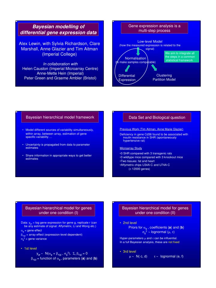
Low-level Model

(how the measured expression is related to the signal)

Normalisation

(to make samples comparable)

Differential Expression Clustering Partition Model

Gene expression analysis is a multi-step process

We aim to integrate all the steps in a common statistical framework

Bayesian hierarchical model framework

• Model different sources of variability simultaneously,

within array, between array, estimation of gene specific variability …

• Uncertainty is propagated from data to parameter

estimates

• Share information in appropriate ways to get better

estimates

Data Set and Biological question

Previous Work (Tim Aitman, Anne Marie Glazier) Deficiency in gene Cd36 found to be associated with insulin resistance in SHR (spontaneously hypertensive rat) Microarray Study

• 3 SHR compared with 3 transgenic rats
• 3 wildtype mice compared with 3 knockout mice
• Two tissues: fat and heart
• Affymetrix chips U34A-C and U74A-C

(≅ 12000 genes) Data: ygr = log gene expression for gene g, replicate r (can be any estimate of signal: Affymetrix, Li and Wong etc.) αg = gene effect βr(g) = array effect (expression-level dependent) σg

2 = gene variance

• 1st level

ygr ∼ N(αg + βr(g) , σg2), Σr βr(g) = 0 βr(g) = function of αg , parameters {a} and {b}

Bayesian hierarchical model for genes under one condition (I)

• 2nd level

Priors for αg , coefficients {a} and {b} σg2 ∼ lognormal (µ, τ)

Hyper-parameters µ and τ can be influential. In a full Bayesian analysis, these are not fixed

• 3rd level

µ ∼ N( c, d) τ ∼ lognormal (e, f)

Bayesian hierarchical model for genes under one condition (II)

We will discuss:

• Array effects (normalisation)
• Bayesian model checks on gene variances
• Confounding of differential and array effects
• Rank statistics

Details of array effects

Exploratory work shows need for expression-level dependent normalisation

Piecewise polynomial with unknown break points: βr(g) = quadratic in αg for ark-1 ≤ αg ≤ ark with coeff (brk(1), brk(2) ), k =1, … #breakpoints

• Locations of break points not fixed
• Must do sensitivity checks on # break points
• Cubic fits well for this data

Non linear fit of array effect as a function

• f gene effect

loess cubic Before (ygr) After (ygr- βr(g) ) Wildtype Knockout

Effect of normalisation on density

^

• Variances are

estimated using information from all G x R measurements (~12000 x 3) rather than just 3

• Variances are

stabilised and shrunk towards average variance

Smoothing of the gene specific variances

• Check our assumptions on gene variances

Bayesian Model Checking

• Predict sample variance Sg

2 new from the model for

each gene

• Compare predicted Sg

2 new with observed Sg 2 obs

Bayesian p-value Prob( Sg

2 new > Sg 2 obs )

• Distribution of p-values Uniform if model is adequate
• Easily implemented in MCMC algorithm

Bayesian predictive p-values

Exchangeable variance model is supported by the data Control for method: equal variance model has too little variability for the data

Differential expression model

dg = differential effect for gene g between 2 conditions Joint model for the 2 conditions : yg1r ∼ N(αg - ½ dg + βr(g)1 , σg12), (condition 1) yg2r ∼ N(αg + ½ dg + βr(g)2 , σg22), (condition 2) So E(yg2 – yg1 ) = dg Prior can be put on dg directly

Possible Statistics for Differential Expression

dg ≈ log fold change dg* = dg / (σ2 g1 / 3 + σ2 g2 / 3 )½ (standardised difference)

• We obtain the joint distribution of all {dg} and/or {dg* }
• Distributions of ranks

Credibility intervals for ranks

150 genes with lowest rank Even genes with median rank less than 100 can have large uncertainty Ranks of modelled log fold change

Probability statements about ranks

Under-expression: probability that gene is ranked in bottom 100 genes Have to choose rank cutoff (here 100) Have to choose how confident we want to be in saying the rank is less than the cutoff (eg prob=80%)

• Model different sources of variability in a single model
• Borrow information from all genes to stabilise estimates of

gene specific variances

• Use joint distribution of ranks for inference
• Future work: mixture prior on log fold changes, with

uncertainty propagated to mixture parameters

Summary