[PPT] - Banks, Money and the Zero Lower Bound on Deposit Rates Michael PowerPoint Presentation

SLIDE 1

Motivation Related Literature The Model Simulations Conclusion

Banks, Money and the Zero Lower Bound

n Deposit Rates

Michael Kumhof1 Xuan Wang 2

3rd Research Conference of CEPR MMCN3 14 June, 2019

1Bank of England 2Presenter, PhD candidate in Financial Economics, Saïd Business School and Exeter

College, University of Oxford

3The views expressed herein are those of the authors and should not be attributed

to the Bank of England

SLIDE 2

Motivation Related Literature The Model Simulations Conclusion

Outline

1 Motivation 2 Related Literature 3 The Model 4 Simulations 5 Conclusion Xuan Wang 1/27

SLIDE 3

Motivation Related Literature The Model Simulations Conclusion

Motivation

◮ 2007-2009 Financial Crisis : macro-finance implication of banks’ balance sheet transformation for credit and liquidity provision. ◮ The need to break the dichotomy between price stability and money & banking, and model banks explicitly (see, e.g. Woodford 2010, Gu et al. 2016). ◮ Problem: recent models use the intermediation of loanable funds theory.

◮ Banks are intermediaries between savers and borrowers of goods and physical capital

◮ Nonfinancial models. ◮ Banks are warehouses of goods. ◮ Commodity money and barter.

◮ Limited scope for the role of credit in liquidity provision (see discussions in

Piazzesi and Schneider 2018, Bianchi and Bigio 2018). Xuan Wang 2/27

SLIDE 4

Motivation Related Literature The Model Simulations Conclusion

Motivation

◮ Solution: Use financing through money creation models.

◮ Banks are creators and intermediaries of money. ◮ Every transaction corresponds to banks’ liability ledger entries. ◮ Support from papers by central banks and policy institutes: BoE (2014, 2018),

Bundesbank (2017), BIS (2011, 2015), RBA (2018), IMF(2014a, b), CBI (2017), Norges Bank (2017), PBoC (2018) .

◮ Support from historical and anthropological evidence: David Graeber (2012). ◮ Proponent: Jakab and Kumhof (2015), Gersbach and Faure (2018).

Xuan Wang 3/27

SLIDE 5

Motivation Related Literature The Model Simulations Conclusion

The Big Picture

◮ Standard decentralised neoclassical model in a nutshell. ◮ What is missing?

◮ What does the firm use to buy L and K? ◮ Implicitly involves contracts & credit risks (household VS firm). ◮ Firm issues bonds and equity to the household; household holds claims (Finance, security design). ◮ However, with multiple goods, security design is not straightforward. ◮ Hence, financing via intermediation: "commercial banks as creators of money" à la Tobin (1963).

Xuan Wang 4/27

SLIDE 6

Motivation Related Literature The Model Simulations Conclusion

The Big Picture

Bank financing in a nutshell ⇒ Inside money: money issued against an offsetting credit that guarantees money’s departure, à la Shubik (1973), Grandmont and Younes (1972, 1973) Shubik and

Tsomocos (1992), Dubey and Geanakoplos (1992, 2003, 2006), Drèze and Polemarchakis (2000).

⇒ Credit risks and financial fragility.

Xuan Wang 5/27

SLIDE 7

Motivation Related Literature The Model Simulations Conclusion

Claiming Niche

◮ What does this paper do? ⇒ DSGE + inside money +nominal rigidities (New Keynesian Financing Model) ⇒ Both credit supply and credit demand ⇒ Shed light on the post-crisis debate on monetary policy effectiveness at the low interest environment (see Brunnermeier and Koby 2019) ZLB: deposit rate ZLB ⇒ constrains policy rate from falling as much as desired

◮ Among the first try to incorporate credit and inside money provision in a dynamic general equilibrium. ◮ Points to the possibility of contractionary policy rate reduction at the ZLB. ◮ A banking/financial explanation for the flattening of the Phillips curve at the ZLB.

Xuan Wang 6/27

SLIDE 8

Motivation Related Literature The Model Simulations Conclusion

Outline

1 Motivation 2 Related Literature 3 The Model 4 Simulations 5 Conclusion Xuan Wang 7/27

SLIDE 9

Motivation Related Literature The Model Simulations Conclusion

Literature - credit and inside money

◮ Money as a financing outcome of credit

◮ Early wisdom: Macleod (1866), Wicksell (1906), Hahn (1920), Hawtrey (1919),

Schumpeter (1934, 1954), Keynes (1931), and Tobin (1963).

◮ Early formalisation in general equilibrium theory: Shubik and Wilson

(1977), Dubey and Geanakoplos (1992, 2003, 2006), Shubik and Tsomocos (1992), Tsomocos (2003), Bloise and Polemarchakis (2006), Goodhart et al. (2006).

◮ Post-crisis: Gu et al. (2016), Bianchi and Bigio (2018), Donaldson et al. (2018),

Bigio and Weill (2016), Brunnermeier and Sannikov (2016), Lagos et al. (2017), Piazzesi and Schneider (2018), McMahon et al. (2018), Tsomocos and Wang (2019), Lagos and Zhang (2019).

Xuan Wang 8/27

SLIDE 10

Motivation Related Literature The Model Simulations Conclusion

Literature

◮ Income, credit and purchasing power:

◮ Post-Keynesian literature: Minsky(1977), Moore (1979), Lavoie (2014), Keen

(2014, 2015).

◮ Contractionary monetary easing near ZLB:

◮ Theory: Brunnermeier and Koby (2018), Eggertsson et al. (2017) ◮ Empirical: Landier et al. (2013), Heider et al. (2017), many others.

◮ Flatter Philips curves near ZLB:

◮ Anchoring of inflation expectations: Blanchard et al. (2015), Blanchard

(2016), Kiley (2015), Ball and Mazumder. (2011).

◮ Real shocks: Leduc and Wilson (2017), Laseen/Sanjani (2016). ◮ Structural change: Gordon (2013), Christiano et al. (2015), many others. ◮ Financial frictions: Gilchrist et al. (2017), focusing on high spreads during

crisis.

Xuan Wang 9/27

SLIDE 11

Motivation Related Literature The Model Simulations Conclusion

Outline

1 Motivation 2 Related Literature 3 The Model 4 Simulations 5 Conclusion Xuan Wang 10/27

SLIDE 12

Motivation Related Literature The Model Simulations Conclusion

Model Overview

◮ Agents: banks, firms, households, government. ◮ Intertemporal linkages:

◮ Government bonds. ◮ Physical capital.

◮ Intratemporal linkages:

◮ Sequence of deposits-in-advance constraints (= budget constraints). ◮ Deposits first created for firms (= borrowers). ◮ Firms pay deposits to households for inputs. ◮ Households pay some deposits to government. ◮ Households and government spend all deposits on firm output. ◮ Firms repay loans in full

◮ No commodity money ◮ Price level determinacy:

◮ Price theory of money à la Calvo (2012, 2016). ◮ Alternatives: outside money à la Dubey and Geanakoplos (1992, 2003, 2006), default à la Lin et al. (2016) , fiscal theory of price level determinacy à la Sims, Cochrane.

Xuan Wang 11/27

SLIDE 13

Motivation Related Literature The Model Simulations Conclusion

Model Overview

Xuan Wang 12/27

SLIDE 14

Motivation Related Literature The Model Simulations Conclusion

Model Overview

Xuan Wang

13/27

SLIDE 15

Motivation Related Literature The Model Simulations Conclusion

Banks

◮ Banks alone can commit to repay. ◮ Banks’s profits = lending spread - cost of lending. ◮ Lending spread (charged to firms): R(Lt) =

it − id

t

Lt

◮ it = lending rate = arbitraged with policy rate. ◮ id

t = deposit rate: Flexible away from ZLB. Stuck at 1 at the ZLB.

◮ Cost of lending: C(Lt) = 1 − β 1 + 1

ξ

Ptℓtgt

t

Lt

Ptℓtgt

t

1+ 1

ξ

⇒ ℓt = ℓtgt

t

it − id

t

1 − β ξ

◮ Upward-sloping loan supply curve. ◮ Not constrained when id

t can adjust.

◮ Highly constrained when id

t = 1 (ZLB).

◮ At ZLB, lowering it directly reduces bank lending.

Xuan Wang 14/27

SLIDE 16

Motivation Related Literature The Model Simulations Conclusion

Empirics for banks

◮ Data and Methodology:

◮ Dependent variable: Log of US real C&I loans. ◮ Explanatory variable: Spread on C&I loans net of smoothed charge-offs. FISIM methodology (Hood (2013)). ◮ Instruments (2SLS):

◮ Lagged % of banks reporting stronger loan demand. ◮ Two alternative instruments yield similar results.

◮ Controls: GDP growth, bank liquidity, tightening bank loan standards.

◮ Result: 1 pp increase in spread associated with 10% increase in loans. ◮ Stylised facts post-GFC:

◮ C&I loan rates dropped with policy rate. ◮ Deposit rates dropped more slowly and then hit ZLB. ◮ Result: Significant spread compression for around 2 years.

Xuan Wang 15/27

SLIDE 17

Motivation Related Literature The Model Simulations Conclusion

Firms

◮ Technology (standard Cobb-Douglas): yt(j) = Sa

tht(j)1−αKt(j)α

◮ Sticky goods price inflation GP,t(j) ◮ Deposits-in-advance

◮ Profits (loan spread = cost) ΠF

t (j) = Pt(j)yt(j) − Wtht(j) − Rk tKt(j) − Lt(j)(it − id t ) − PtGP,t(j)

◮ Deposits-in-advance: Lt(j) Lt(j)(it − 1) + Wtht(j) + Rk

tKt(j) + ΠF t (j)

Xuan Wang 16/27

SLIDE 18

Motivation Related Literature The Model Simulations Conclusion

Firms

◮ Lagrangean: Max E0

∞

∑

t=0

βtΛh

t

(Pt(j))1−θ (Pt)θ yt − Wtht(j) − Rk

tKt(j)

−Lt(j)(it − id

t ) − φP

2 Ptyt  

Pt(j) Pt−1(j)

πt−1 − 1  

2

−MCt

(Pt(j))−θ (Pt)θ yt − Sa

tht(j)1−αKt(j)α

+ηf

t

  Lt(j) − (Pt(j))1−θ (Pt)θ yt + φP 2 Ptyt  

Pt(j) Pt−1(j)

πt−1 − 1  

2

  −ηb

t

 Lt(j) − Ptℓtgt

t

it − id

t

1 − β ξ   

Xuan Wang 17/27

SLIDE 19

Motivation Related Literature The Model Simulations Conclusion

Firms

◮ Non-standard optimality conditions:

◮ Phillips curve: µmct (1 − ηf

t )

− 1 = f πt πt−1

− Mt

yt+1 yt (1 − ηf

t+1)

(1 − ηf

t )

f πt+1 πt

= 0

◮ Loans FOC: it − id

t = ηf t − ηb t

◮ Away from the ZLB: 1 − ηf

t = 1 − it + id t . Deposit rate enters.

◮ At the ZLB: 1 − ηf

t = 2 − it − ηb t . Credit rationing multiplier enters.

Xuan Wang 18/27

SLIDE 20

Motivation Related Literature The Model Simulations Conclusion

The household

◮ Standard household problem with a twist. ◮ Lifetime utility: Max

{ct(i),ht(i),It(i),kt(i),Bt(i)}∞

t=0

E0

∞

∑

t=0

βt[Sc

t(1 − v)

1 ǫ (ct(i) − vct−1)1− 1 ǫ

1 − 1

ǫ

− χ 2 ht(i)2] ◮ Capital accumulation: kt = (1 − δ) kt−1 + It ◮ Budget constraint: Bt−1(i) + Wtht(i)(1 − τL,t) + Rk

tkt−1(i) + Dhb t + Dhm t

+ Bt(i)(it − 1) ≥ Ptct(i) + PtIt(i) + PtGI,t(i) + Bt(i) ◮ Twist: This budget constraint can be shown to be an intra-period deposits-in-advance constraint, and deposits are not endowed.

Xuan Wang 19/27

SLIDE 21

Motivation Related Literature The Model Simulations Conclusion

Government

◮ Budget constraint: Bt = Bt−1 + Bt (it − 1) + Ptgt − τL,tWtht ◮ Fiscal rule: τL,t − ¯ τL = fb bt 4yt − bss 4yss

◮ Monetary policy rule:

it = ((2 − β) ¯ π) πt ¯ π mπ

Xuan Wang 20/27

SLIDE 22

Motivation Related Literature The Model Simulations Conclusion

Outline

1 Motivation 2 Related Literature 3 The Model 4 Simulations 5 Conclusion Xuan Wang 21/27

SLIDE 23

Motivation Related Literature The Model Simulations Conclusion

Figure 1: Calibration

Xuan Wang 22/27

SLIDE 24

Motivation Related Literature The Model Simulations Conclusion

0.9
0.8
0.7
0.6
0.5
0.4
0.3
0.2
0.1

0.0

0.9
0.8
0.7
0.6
0.5
0.4
0.3
0.2
0.1

0.0 0 2 4 6 8 10 12 14 16 18 20

GDP

(% Difference)

1.4
1.2
1.0
0.8
0.6
0.4
0.2
0.0
1.4
1.2
1.0
0.8
0.6
0.4
0.2
0.0

0 2 4 6 8 10 12 14 16 18 20

Consumption

(% Difference)

0.4
0.2

0.0 0.2 0.4 0.6 0.8 1.0

0.4
0.2

0.0 0.2 0.4 0.6 0.8 1.0 0 2 4 6 8 10 12 14 16 18 20

Investment

(% Difference)

0.9
0.8
0.7
0.6
0.5
0.4
0.3
0.2
0.1

0.0

0.9
0.8
0.7
0.6
0.5
0.4
0.3
0.2
0.1

0.0 0 2 4 6 8 10 12 14 16 18 20

Bank Loans

(% Difference)

0.10
0.09
0.08
0.07
0.06
0.05
0.04
0.03
0.02
0.01
0.00
0.10
0.09
0.08
0.07
0.06
0.05
0.04
0.03
0.02
0.01
0.00

0 2 4 6 8 10 12 14 16 18 20

Inflation Rate

(pp Difference)

0.40
0.35
0.30
0.25
0.20
0.15
0.10
0.05

0.00

0.40
0.35
0.30
0.25
0.20
0.15
0.10
0.05

0.00 0 2 4 6 8 10 12 14 16 18 20

Nominal Policy Rate

(pp Difference)

0.10
0.08
0.06
0.04
0.02
0.00

0.02 0.04 0.06 0.08 0.10

0.10
0.08
0.06
0.04
0.02
0.00

0.02 0.04 0.06 0.08 0.10 0 2 4 6 8 10 12 14 16 18 20

Nominal Deposit Rate

(pp Difference)

0.40
0.35
0.30
0.25
0.20
0.15
0.10
0.05

0.00

0.40
0.35
0.30
0.25
0.20
0.15
0.10
0.05

0.00 0 2 4 6 8 10 12 14 16 18 20

Nominal Lending Spread

(pp Difference)

0.25
0.20
0.15
0.10
0.05

0.00

0.25
0.20
0.15
0.10
0.05

0.00 0 2 4 6 8 10 12 14 16 18 20

MC - Total

(% Difference) 0.0 0.2 0.4 0.6 0.8 1.0 1.2 1.4 1.6 0.0 0.2 0.4 0.6 0.8 1.0 1.2 1.4 1.6 0 2 4 6 8 10 12 14 16 18 20

MC - Credit Rationing

(% Difference)

1.6
1.4
1.2
1.0
0.8
0.6
0.4
0.2

0.0

1.6
1.4
1.2
1.0
0.8
0.6
0.4
0.2

0.0 0 2 4 6 8 10 12 14 16 18 20

MC - Capital and Labor

(% Difference)

0.30
0.25
0.20
0.15
0.10
0.05
0.00
0.30
0.25
0.20
0.15
0.10
0.05
0.00

0 2 4 6 8 10 12 14 16 18 20

Real Policy Rate

(pp Difference)

Figure 2: CD shock Policy Rate Contraction, semi-elasticities: solid=10,

dashed =5, dotted =1 Xuan Wang 23/27

SLIDE 25

Motivation Related Literature The Model Simulations Conclusion

0.9
0.8
0.7
0.6
0.5
0.4
0.3
0.2
0.1

0.0

0.9
0.8
0.7
0.6
0.5
0.4
0.3
0.2
0.1

0.0 0 2 4 6 8 10 12 14 16 18 20

GDP

(% Difference)

1.4
1.2
1.0
0.8
0.6
0.4
0.2
0.0
1.4
1.2
1.0
0.8
0.6
0.4
0.2
0.0

0 2 4 6 8 10 12 14 16 18 20

Consumption

(% Difference) 0.0 0.5 1.0 1.5 0.0 0.5 1.0 1.5 0 2 4 6 8 10 12 14 16 18 20

Investment

(% Difference)

0.9
0.8
0.7
0.6
0.5
0.4
0.3
0.2
0.1

0.0

0.9
0.8
0.7
0.6
0.5
0.4
0.3
0.2
0.1

0.0 0 2 4 6 8 10 12 14 16 18 20

Bank Loans

(% Difference)

0.12
0.10
0.08
0.06
0.04
0.02

0.00

0.12
0.10
0.08
0.06
0.04
0.02

0.00 0 2 4 6 8 10 12 14 16 18 20

Inflation Rate

(pp Difference)

0.50
0.45
0.40
0.35
0.30
0.25
0.20
0.15
0.10
0.05

0.00

0.50
0.45
0.40
0.35
0.30
0.25
0.20
0.15
0.10
0.05

0.00 0 2 4 6 8 10 12 14 16 18 20

Nominal Policy Rate

(pp Difference)

0.45
0.40
0.35
0.30
0.25
0.20
0.15
0.10
0.05

0.00

0.45
0.40
0.35
0.30
0.25
0.20
0.15
0.10
0.05

0.00 0 2 4 6 8 10 12 14 16 18 20

Nominal Deposit Rate

(pp Difference)

0.07
0.06
0.05
0.04
0.03
0.02
0.01
0.00
0.07
0.06
0.05
0.04
0.03
0.02
0.01
0.00

0 2 4 6 8 10 12 14 16 18 20

Nominal Lending Spread

(pp Difference)

0.10
0.05

0.00 0.05 0.10

0.10
0.05

0.00 0.05 0.10 0 2 4 6 8 10 12 14 16 18 20

MC - Total

(% Difference) 0.0 0.2 0.4 0.6 0.8 1.0 1.2 1.4 1.6 0.0 0.2 0.4 0.6 0.8 1.0 1.2 1.4 1.6 0 2 4 6 8 10 12 14 16 18 20

MC - Credit Rationing

(% Difference)

1.6
1.4
1.2
1.0
0.8
0.6
0.4
0.2

0.0

1.6
1.4
1.2
1.0
0.8
0.6
0.4
0.2

0.0 0 2 4 6 8 10 12 14 16 18 20

MC - Capital and Labor

(% Difference)

0.40
0.35
0.30
0.25
0.20
0.15
0.10
0.05

0.00

0.40
0.35
0.30
0.25
0.20
0.15
0.10
0.05

0.00 0 2 4 6 8 10 12 14 16 18 20

Real Policy Rate

(pp Difference)

Figure 3: CD Shock - Flat Phillips Curve, ZLB constrained (dashed) versus

unconstrained (dotted) Xuan Wang 24/27

SLIDE 26

Motivation Related Literature The Model Simulations Conclusion

0.0 0.5 1.0 1.5 2.0 2.5 3.0 3.5 4.0 0.0 0.5 1.0 1.5 2.0 2.5 3.0 3.5 4.0 0 4 8 12 16 20 24 28 32 36 40

GDP

(% Difference) 0.0 0.2 0.4 0.6 0.8 1.0 1.2 1.4 1.6 0.0 0.2 0.4 0.6 0.8 1.0 1.2 1.4 1.6 0 4 8 12 16 20 24 28 32 36 40

Consumption

(% Difference) 2 4 6 8 10 12 14 16 2 4 6 8 10 12 14 16 0 4 8 12 16 20 24 28 32 36 40

Investment

(% Difference) 0.0 0.5 1.0 1.5 2.0 2.5 3.0 3.5 4.0 0.0 0.5 1.0 1.5 2.0 2.5 3.0 3.5 4.0 0 4 8 12 16 20 24 28 32 36 40

Bank Loans

(% Difference) 0.00 0.05 0.10 0.15 0.20 0.25 0.30 0.35 0.00 0.05 0.10 0.15 0.20 0.25 0.30 0.35 0 4 8 12 16 20 24 28 32 36 40

Inflation Rate

(pp Difference)

0.2
0.1

0.0 0.1 0.2 0.3 0.4 0.5 0.6

0.2
0.1

0.0 0.1 0.2 0.3 0.4 0.5 0.6 0 4 8 12 16 20 24 28 32 36 40

Nominal Policy Rate

(pp Difference)

0.25
0.20
0.15
0.10
0.05

0.00 0.05 0.10 0.15 0.20 0.25

0.25
0.20
0.15
0.10
0.05

0.00 0.05 0.10 0.15 0.20 0.25 0 4 8 12 16 20 24 28 32 36 40

Nominal Deposit Rate

(pp Difference) 0.0 0.1 0.2 0.3 0.4 0.5 0.6 0.0 0.1 0.2 0.3 0.4 0.5 0.6 0 4 8 12 16 20 24 28 32 36 40

Nominal Lending Spread

(pp Difference) 0.0 0.1 0.2 0.3 0.4 0.5 0.6 0.7 0.8 0.9 0.0 0.1 0.2 0.3 0.4 0.5 0.6 0.7 0.8 0.9 0 4 8 12 16 20 24 28 32 36 40

MC - Total

(% Difference)

7
6
5
4
3
2
1
7
6
5
4
3
2
1

0 4 8 12 16 20 24 28 32 36 40

MC - Credit Rationing

(% Difference) 1 2 3 4 5 6 7 8 1 2 3 4 5 6 7 8 0 4 8 12 16 20 24 28 32 36 40

MC - Capital and Labor

(% Difference)

0.4
0.3
0.2
0.1

0.0 0.1 0.2 0.3

0.4
0.3
0.2
0.1

0.0 0.1 0.2 0.3 0 4 8 12 16 20 24 28 32 36 40

Real Policy Rate

(pp Difference)

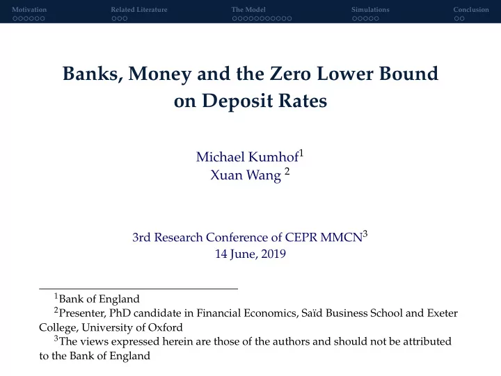
Figure 4: CD Shock - piebar, ZLB constrained (solid) versus unconstrained

(dashed) Xuan Wang 25/27

SLIDE 27

Motivation Related Literature The Model Simulations Conclusion

Outline

1 Motivation 2 Related Literature 3 The Model 4 Simulations 5 Conclusion Xuan Wang 26/27

SLIDE 28

Motivation Related Literature The Model Simulations Conclusion

Conclusion

◮ Results

◮ Infinite-horizon model of endogenous money creation by banks. ◮ Bank deposits = only money in the economy (no outside money). ◮ Bank deposits created through book entries and exit via loan repayment. ◮ ZLB prevents banks from elastically supplying money. ◮ Phillips curve turns out flatter at the ZLB due to the credit constraint.

◮ A broader role

◮ An attempt to bridge the gap between money and banking and the real business cycle literature. ◮ Ties money and liquidity with credit and opens the avenue for financial stability analysis.

◮ Future avenues

◮ Explicitly model credit risks via strategic default. ◮ Interact money and price stability with financial stability risks (see Tsomocos and Wang 2019 and Goodhart et al. 2019). ◮ Flexible prices, value for money, seigniorage and default.

Xuan Wang 27/27