Ba sic Skill of Ma c hine L e a rning with MAT L AB Stanley - - PDF document

7/26/2017 1

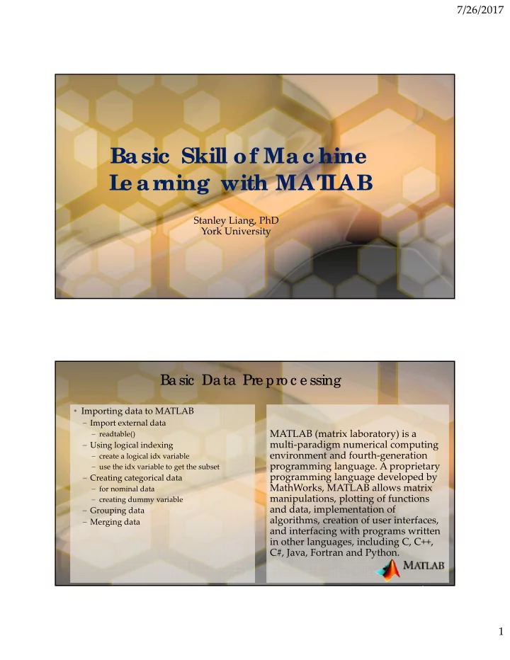
Ba sic Skill of Ma c hine L e a rning with MAT L AB

Stanley Liang, PhD York University

Basic Data Pre pro c e ssing

MATLAB (matrix laboratory) is a multi‐paradigm numerical computing environment and fourth‐generation programming language. A proprietary programming language developed by MathWorks, MATLAB allows matrix manipulations, plotting of functions and data, implementation of algorithms, creation of user interfaces, and interfacing with programs written in other languages, including C, C++, C#, Java, Fortran and Python.

• Importing data to MATLAB

– Import external data

– readtable()

– Using logical indexing

– create a logical idx variable – use the idx variable to get the subset

– Creating categorical data

– for nominal data – creating dummy variable

– Grouping data – Merging data

7/26/2017 2

Visualize Data fo r F irst I mpre ssio n

• Boxplot
• Scatter

No rmalizing Data

• Many of the clustering methods use the distance between the observations

as a similarity measure. Smaller distances indicate more similar

• bservations.
• In the patient dataset, the systolic pressure is likely to be higher than the

diastolic pressure. However, diastolic pressure > 90 mmHg is hypertension, but systolic pressure >120 mmHg is still normal

• Each statistic has different units and scales. When using the distance

measure, statistics with wider scales will be given more importance

7/26/2017 3

Unsupe rvise d L e arning

I de ntifying Gro ups by Visualizing the Data

• A quick way to group data is to visualize the data and see if there

are any obvious patterns and groups

• To effectively visualize the data containing more than three

predictors, we can use the dimensionality reduction techniques such as multidimensional scaling and principal component analysis (PCA).

7/26/2017 4

Multidime nsio nal Sc aling

• 1. Calculate pairwise distances

– d = pdist(measurements, distance) – d: a distance or dissimilarity vector containing the distance between each pair of

• bservations

– measurements ‐‐ A numeric matrix containing the data. Each row is considered as an observation – distance ‐‐ An optional input that indicates the method of calculating the dissimilarity or distance. Commonly used methods are ʹeuclideanʹ (default), ʹcityblockʹ, and ʹcorrelation

2. Perform multidimensional scaling

– [x, e] = cmdscale(d) – x ‐‐ The m‐by‐q matrix of the reconstructed coordinates in q‐dimensional space. q is the minimum number of dimensions needed to achieve the given pairwise distances. – e ‐‐ Eigenvalues of the matrix x*x‘ – d ‐‐ A dissimilarity or distance vector

Princ ipal Co mpo ne nt Analysis

• Principal component analysis (PCA) is a popular method for

dimensionality reduction

• The MATLAB provides the pca() function for PCA

– [pcs ,scrs,~,~,pexp] = pca(measurements) – pcs ‐‐ A n‐by‐n matrix of principal components. – scrs ‐‐ A matrix containing the data transformed using the linear coordinate transformation matrix pcs – pexp ‐‐ A vector of the percentage of variance explained by each principal component – measurements ‐‐ A numeric matrix containing n columns corresponding to the the observed variables. Each row corresponds to an observation.

7/26/2017 5

k-me ans Cluste ring

• By on the result of PCA and multidimensional scaling, we get the initial

impression that the data can be grouped by 2

• Then we can use the k‐means clustering method to divide the observations into

groups or clusters

• MATLAB function for k‐means clustering

– idx = kmeans(X,k) – idx ‐‐ Cluster indices, returned as a numeric column vector. – X ‐‐ Data, specified as a numeric matrix – k ‐‐ Number of clusters.

• There are several options to tune the clustering, the default method is euclidean

distance

• Another way to get optimum clustering is to perform the analysis multiple times

with different starting centroids and then choose the clustering scheme which minimizes the sum of distances between the centroids and the observations (sumd).

Cluste ring by Gaussian Mixture Mo de l

• Gaussian Mixture Models (GMM) clustering involves fitting several

n‐dimensional normal distributions to the data

• 1. Fit Gaussian Mixture Model ‐‐ fitgmdist

– it fits several multidimensional gaussian (normal) distributions – gmdl = fitgmdist(data,4) ‐‐ fit 4 distributions

• 2. Identify Clusters ‐ calculate each observation’s posterior

probability for each component

– grps = cluster(gmdl,data); – [grps,~,p] = cluster(gmdl,X); ‐‐get the probability

• 3. Visualize the result

7/26/2017 6

I nte rpre ting the Cluste rs

• Visualizing Observations in Clusters

–With high‐dimensional data, it is difficult to visualize the groups as points in space – Use of the parallelcoords() function –parallelcoords(X,ʹGroupʹ,g)

–x ‐‐ Data, specified as a numeric matrix. – ʹGroupʹ ‐‐ Property Name. –g ‐‐ A vector containing the cluster identifiers.

E valuating Cluste r Quality

• When using clustering techniques such as k‐means and Gaussian mixture

model, you have to specify the number of clusters.

• However, for high dimensional data, it is difficult to determine the optimum

number of clusters.

• An observation’s silhouette value is a normalized (between ‐1 and +1)

measure of how close that observation is to others in the same cluster, compared to the observations in different clusters.

• Silhouette Plots

– shows the silhouette value of each observation, grouped by cluster – Clustering schemes in which most of the observations have high silhouette value are desirable

7/26/2017 7

Auto mate Cluste r Quality E valuatio n

• Instead of manually experimenting with silhouette plots with

different number of clusters, you can automate the process with evalclusters function.

• the evalclusters() function

– creates m to n clusters by a defined method – computes the silhouette value for each clustering scheme