> b x 2 w 3 x 3 Neuroscience 101 CMPSCI 689 Subhransu Maji - - PowerPoint PPT Presentation

Subhransu Maji

3 February 2015

CMPSCI 689: Machine Learning

5 February 2015

Perceptron

Subhransu Maji (UMASS) CMPSCI 689 /19

Decision trees!

• Inductive bias: use a combination of small number of features!

Nearest neighbor classifier!

• Inductive bias: all features are equally good

Perceptrons Today!

• Inductive bias: use all features, but some more than others

So far in the class

2 Subhransu Maji (UMASS) CMPSCI 689 /19

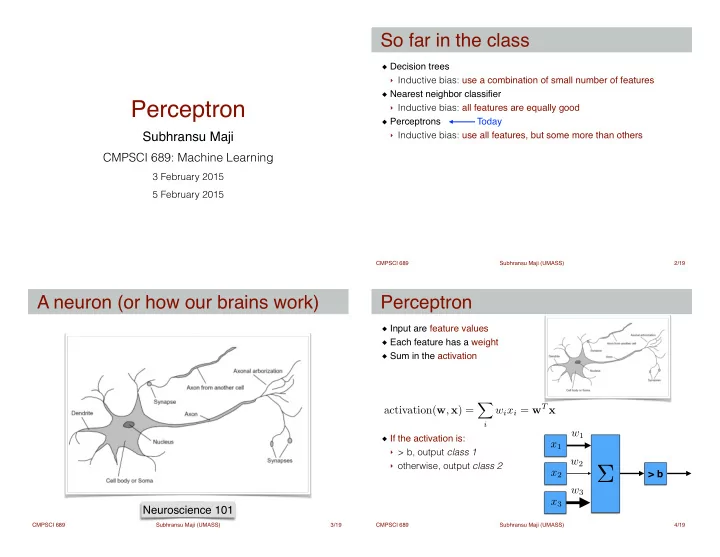
A neuron (or how our brains work)

3

Neuroscience 101

Subhransu Maji (UMASS) CMPSCI 689 /19

Input are feature values! Each feature has a weight! Sum in the activation!

! ! ! ! !

If the activation is:!

• > b, output class 1
• otherwise, output class 2

Perceptron

4

> b

Σ

w1 w2 w3 x3 x2 x1 activation(w, x) = X

i

wixi = wT x

Subhransu Maji (UMASS) CMPSCI 689 /19

Input are feature values! Each feature has a weight! Sum in the activation!

! ! ! ! !

If the activation is:!

• > b, output class 1
• otherwise, output class 2

Perceptron

4

> b

Σ

w1 w2 w3 x3 x2 x1 activation(w, x) = X

i

wixi = wT x x → (x, 1) wT x + b → (w, b)T (x, 1)

Subhransu Maji (UMASS) CMPSCI 689 /19

Imagine 3 features (spam is “positive” class):!

• free (number of occurrences of “free”)
• money (number of occurrences of “money”)
• BIAS (intercept, always has value 1)

Example: Spam

5

email w x wT x wT x > 0 → SPAM!!

Subhransu Maji (UMASS) CMPSCI 689 /19

In the space of feature vectors!

• examples are points (in D dimensions)
• an weight vector is a hyperplane (a D-1 dimensional object)
• One side corresponds to y=+1
• Other side corresponds to y=-1

Perceptrons are also called as linear classifiers

Geometry of the perceptron

6

w wT x = 0

Subhransu Maji (UMASS) CMPSCI 689 /19

Initialize ! for iter = 1,…,T!

• for i = 1,..,n!
• predict according to the current model!

! ! !

• if , no change!
• else,

Learning a perceptron

7

yi = ˆ yi w ← w + yixi w ← [0, . . . , 0] (x1, y1), (x2, y2), . . . , (xn, yn) Input: training data

Perceptron training algorithm [Rosenblatt 57]

xi w yix ˆ yi = ⇢ +1 if wT xi > 0 −1 if wT xi ≤ 0 yi = −1

Subhransu Maji (UMASS) CMPSCI 689 /19

Initialize ! for iter = 1,…,T!

• for i = 1,..,n!
• predict according to the current model!

! ! !

• if , no change!
• else,

Learning a perceptron

7

yi = ˆ yi w ← w + yixi w ← [0, . . . , 0] (x1, y1), (x2, y2), . . . , (xn, yn) Input: training data

Perceptron training algorithm [Rosenblatt 57]

xi w yix ˆ yi = ⇢ +1 if wT xi > 0 −1 if wT xi ≤ 0 error driven, online, activations increase for +, randomize yi = −1

Subhransu Maji (UMASS) CMPSCI 689 /19

Separability: some parameters will classify the training data perfectly!

!

Convergence: if the training data is separable then the perceptron training will eventually converge [Block 62, Novikoff 62]!

!

Mistake bound: the maximum number of mistakes is related to the margin

Properties of perceptrons

8

#mistakes <

1 δ2

assuming, ||xi|| ≤ 1 δ = maxw min(xi,yi) ⇥ yiwT xi ⇤ such that, ||w|| = 1

Subhransu Maji (UMASS) CMPSCI 689 /19

Review geometry

9 Subhransu Maji (UMASS) CMPSCI 689 /19

Proof of convergence

10

Let,ˆ w be the separating hyperplane with margin δ

Subhransu Maji (UMASS) CMPSCI 689 /19

Proof of convergence

10

ˆ wT w(k) = ˆ wT ⇣ w(k−1) + yixi ⌘ = ˆ wT w(k−1) + ˆ wT yixi ≥ ˆ wT w(k−1) + δ ≥ kδ ||w(k)|| ≥ kδ

update rule algebra definition of margin w is getting closer

Let,ˆ w be the separating hyperplane with margin δ

Subhransu Maji (UMASS) CMPSCI 689 /19

Proof of convergence

10

||w(k)||2 = ||w(k−1) + yixi||2 ≤ ||w(k−1)||2 + ||yixi||2 ≤ ||w(k−1)||2 + 1 ≤ k ||w(k)|| ≤ √ k

update rule triangle inequality norm bound the norm

ˆ wT w(k) = ˆ wT ⇣ w(k−1) + yixi ⌘ = ˆ wT w(k−1) + ˆ wT yixi ≥ ˆ wT w(k−1) + δ ≥ kδ ||w(k)|| ≥ kδ

update rule algebra definition of margin w is getting closer

Let,ˆ w be the separating hyperplane with margin δ

Subhransu Maji (UMASS) CMPSCI 689 /19

Proof of convergence

10

kδ ≤ ||w(k)|| ≤ √ k − → k ≤ 1 δ2 ||w(k)||2 = ||w(k−1) + yixi||2 ≤ ||w(k−1)||2 + ||yixi||2 ≤ ||w(k−1)||2 + 1 ≤ k ||w(k)|| ≤ √ k

update rule triangle inequality norm bound the norm

ˆ wT w(k) = ˆ wT ⇣ w(k−1) + yixi ⌘ = ˆ wT w(k−1) + ˆ wT yixi ≥ ˆ wT w(k−1) + δ ≥ kδ ||w(k)|| ≥ kδ

update rule algebra definition of margin w is getting closer

Let,ˆ w be the separating hyperplane with margin δ

Subhransu Maji (UMASS) CMPSCI 689 /19

Convergence: if the data isn’t separable, the training algorithm may not terminate!

• noise can cause this
• some simple functions are not

separable (xor)

!

Mediocre generation: the algorithm finds a solution that “barely” separates the data!

!

Overtraining: test/validation accuracy rises and then falls!

• Overtraining is a kind of overfitting

Limitations of perceptrons

11

Subhransu Maji (UMASS) CMPSCI 689 /19

Problem: updates on later examples can take over!

• 10000 training examples
• The algorithm learns weight vector on the first 100 examples
• Gets the next 9899 points correct
• Gets the 10000th point wrong, updates on the the weight vector
• This completely ruins the weight vector (get 50% error)

! ! ! ! ! ! !

Voted and averaged perceptron (Freund and Schapire, 1999)

A problem with perceptron training

12

w(9999) w(10000) x10000

Subhransu Maji (UMASS) CMPSCI 689 /19

Let, , be the sequence of weights obtained by the perceptron learning algorithm.! Let, , be the survival times for each of these.!

• a weight that gets updated immediately gets c = 1
• a weight that survives another round gets c = 2, etc.

Then,

Voted perceptron

13

w(1), w(2), . . . , w(K) c(1), c(2), . . . , c(K) Key idea: remember how long each weight vector survives ˆ y = sign K X

k=1

c(k)sign ⇣ w(k)T x ⌘!

Subhransu Maji (UMASS) CMPSCI 689 /19

Initialize: ! for iter = 1,…,T!

• for i = 1,..,n!
• predict according to the current model!

! ! !

• if , !
• else,

Voted perceptron training algorithm

14

yi = ˆ yi (x1, y1), (x2, y2), . . . , (xn, yn) Input: training data k = 0, c(1) = 0, w(1) ← [0, . . . , 0] ˆ yi = ⇢ +1 if w(k)T xi > 0 −1 if w(k)T xi ≤ 0 c(k) = c(k) + 1 w(k+1) = w(k) + yixi c(k+1) = 1 k = k + 1 Output: list of pairs (w(1), c(1)), (w(2), c(2)), . . . , (w(K), c(K))

Subhransu Maji (UMASS) CMPSCI 689 /19

Initialize: ! for iter = 1,…,T!

• for i = 1,..,n!
• predict according to the current model!

! ! !

• if , !
• else,

Voted perceptron training algorithm

14

yi = ˆ yi (x1, y1), (x2, y2), . . . , (xn, yn) Input: training data k = 0, c(1) = 0, w(1) ← [0, . . . , 0] ˆ yi = ⇢ +1 if w(k)T xi > 0 −1 if w(k)T xi ≤ 0 c(k) = c(k) + 1 w(k+1) = w(k) + yixi c(k+1) = 1 k = k + 1 Output: list of pairs (w(1), c(1)), (w(2), c(2)), . . . , (w(K), c(K)) Better generalization, but not very practical

Subhransu Maji (UMASS) CMPSCI 689 /19

Let, , be the sequence of weights obtained by the perceptron learning algorithm.! Let, , be the survival times for each of these.!

• a weight that gets updated immediately gets c = 1
• a weight that survives another round gets c = 2, etc.

Then,

Averaged perceptron

15

w(1), w(2), . . . , w(K) c(1), c(2), . . . , c(K) Key idea: remember how long each weight vector survives performs similarly, but much more practical ˆ y = sign K X

k=1

c(k) ⇣ w(k)T x ⌘! = sign ¯ wT x

• Subhransu Maji (UMASS)

CMPSCI 689 /19

Initialize: ! for iter = 1,…,T!

• for i = 1,..,n!
• predict according to the current model!

! ! !

• if , !
• else, !

! !

Return

Averaged perceptron training algorithm

16

yi = ˆ yi (x1, y1), (x2, y2), . . . , (xn, yn) Input: training data Output: ¯ w ← ¯ w + cw c = c + 1 c = 0, w = [0, . . . , 0], ¯ w = [0, . . . , 0] ˆ yi = ⇢ +1 if wT xi > 0 −1 if wT xi ≤ 0 c = 1 w ← w + yixi ¯ w update average ← ¯ w + cw

Subhransu Maji (UMASS) CMPSCI 689 /19

Comparison of perceptron variants

17

MNIST dataset (Figure from Freund and Schapire 1999)

Subhransu Maji (UMASS) CMPSCI 689 /19

Multilayer perceptrons: to learn non-linear functions of the input (neural networks)!

!

Separators with good margins: improves generalization ability of the classifier (support vector machines)

!

Feature-mapping: to learn non-linear functions of the input using a perceptron!

• we will learn do this efficiently using kernels

Improving perceptrons

18

φ : (x1, x2) → (x2

1,

√ 2x1x2, x2

2)

x2

1

a2 + x2

2

b2 = 1 → z1 a2 + z3 b2 = 1

Subhransu Maji (UMASS) CMPSCI 689 /19

Some slides adapted from Dan Klein at UC Berkeley and CIML book by Hal Daume! Figure comparing various perceptrons are from Freund and Schapire

Slides credit

19