min such that y 1 2 Then we have: C q S is created by - PowerPoint PPT Presentation

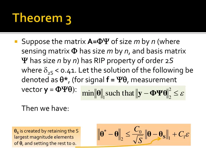
 Suppose the matrix A= FY of size m by n (where sensing matrix F has size m by n , and basis matrix Y has size n by n ) has RIP property of order 2 S where d 2S < 0.41. Let the solution of the following be denoted as q * , (for signal f = Yq , measurement vector y = FYq): 2    θ ΦΨθ min such that y 1 2 Then we have: C q S is created by retaining the S      θ θ θ θ * 0 C largest magnitude elements 1 S 1 2 S of q , and setting the rest to 0.

 The proof can be found in a paper by Candes “The restricted isometry property and its implications for compressed sensing” , published in 2008.  The proof as such is just between 1 and 2 pages long.

 The proof uses various properties of vectors in Euclidean space. v w v w    The Cauchy Schwartz inequality: | | 2 2 v w v w     The triangle inequality: 2 2 2 v w v w     Reverse triangle inequality: 2 2 2

 Relationship between various norms: v v v 1 v     | | n 2 1 2 v v  if is a - sparse vector k k 2  Refer to Theorem 3. For the sake of simplicity alone, we shall assume Y to be the identity matrix.  Hence x = θ . Even if Y were not identity, the proof as such does not change.

This result is called the Tube constraint .  We have: Φ x * x Φx * y Φx y        ( ) 2 0 0 2 2 2 In the following, Given constraint + feasibility Triangle inequality x 0 = true signal of solution x* 2 ε y = Φ x x 0

h x * x    Define vector . 0  Decompose h into vectors h T0 , h T1 , h T2 ,… which are all at the most s -sparse.  T 0 contains indices corresponding to the s largest elements of x , T 1 contains indices corresponding to the s largest elements of h (T0-c) = h - h T0 , T 2 contains indices corresponding to the s largest indices of h (T0 U T1)-c = h - h T0 - h T1 , and so on.

 We will assume x 0 is s-sparse (later we will remove this requirement).  We now establish the so-called cone constraint. The vector h has its origin at x 0    and it lies in the intersection of * x x h x the L1 ball and the tube. 0 0 1 1 1        | | | | x h x h x 0 0 0 i i i i 1 0-valued   i T i T  0 0 c     x h h x The vector h must also  0 0 0 0 T T c 1 1 1 1 necessarily obey this   h h constraint – the cone  0 0 T c T 1 1 constraint.

 We will now prove that such a vector h is orthogonal to the null-space of Φ .   In fact, we will prove that . Φh h 2 2  In other words, we will prove that the magnitude of h is not much greater than 2 ε , which means that the solution x* of the optimization problem is close enough to x 0 .

 In step 3, we use a bunch of algebraic manipulations to prove that the magnitude of h outside of T 0 U T 1 is upper bounded by the magnitude of h on T 0 U T 1 .  In other words, we prove that: h h h   (T0 T1) - c T0 T0 T0 T0 T1 T1   2 2 2  The algebra involves various inequalities mentioned earlier.

 We now prove that the magnitude of h on T 0 U T 1 is upper bounded by a reasonable quantity.  For this, we show using the RIP of Φ of order 2 s and a series of manipulations that: 2 2  d  F    d  d ( 1 ) ( 2 1 2 ) h h h h    2 0 1 0 1 0 1 2 2 0 s T T T T T T s s T 2 2 2 2  This implies that     d  d    d d 2 1 2 1 4 1 2         2 2 2 s 2 s s s h h h h       d  d T 0 T 1 T 0 T 1 T 0 T 1  d   d  2 2 2 1 1 1 ( 2 1 ) 1 ( 2 1 ) 2   2 s 2 s 2 s 2 s

 The steps change a bit. The cone constraint changes to:    * x x h x 0 0 1 1 1        | | | | x h x h x 0 0 0 i i i i 1   i T i T  0 0 c      x h h x x   0 , 0 0 0 0 , 0 0 T T T c T c 1 1 1 1 1    2 h h x   0 0 0 , 0 T c T T c 1 1 1

 All the other steps remain as is, except the last one which produces the following bound:   d  d  x x 2 1 1 ( 2 1 ) 0 0 , 0    T 2 s 2 s 1 h  d   d  2 1 ( 1 2 ) 1 ( 2 1 ) s 2 2 s s

 Step 3 of the proof uses the following corollary of the RIP for two s -sparse unit   d Φx 1 Φx | | vectors with disjoint support: 2 2 s  Proof of corollary: 2 2 2  d      d  Φ ( 1 ) ( ) ( 1 ) , by RIP x x x x x x 2 2 S 1 2 1 2 s 1 2 1 Φ Φ Φ Φ Φ Φ 2 2      | | x x x x x x 1 2 1 2 1 2 4  ) 1   d  2   d  2 ( 1 ) ( 1 ) x x x x 2 2 s 1 2 s 1 2 4  ) 1 2 2 2 2   d      d    ( 1 )( 2 ) ( 1 )( 2 ) x x x x x x x x 2 2 s 1 2 1 2 s 1 2 1 2 4 2 2  d      1 , 0 x x x x 2 1 s 1 2 2

 This step also uses the following corollary of the RIP for two s -sparse unit vectors with   d disjoint support: Φx 1 Φx | | 2 2 s  What if the original vectors x 1 and x 2 were not unit-vectors, but both were s -sparse?  Φx Φx | |  d    d Φx Φx 1 2 | | x x 2 2 s 1 2 s 1 2 2 2 x x 1 2 2 2

 The bound is  d  d  4 1 1 1 ( 2 1 ) h x x     2 s 2 s 0 0, 0, T0 T0   d   d 2 1 1 ( 1 2 ) 1 ( 1 2 ) s 2 2 s s  Note the requirement that δ 2s should be less than 2 0.5 - 1.  You can prove that the two constant factors – one before  and the other before | x 0 - x 0,TO | 1 , are both increasing functions of δ 2s in the domain [0,1].  So sensing matrices with smaller values of δ 2s are always nicer!

 Suppose the matrix A= FY of size m by n (where sensing matrix F has size m by n , and basis matrix Y has size n by n ) has RIP property of order S where d S < 0.307. Let the solution of the following be denoted as q * , (for signal f = Yq , measurement vector y = FYq): 2    θ ΦΨθ min such that y 1 2 Then we have: 1 1      θ θ θ θ *  d  d S 1 0 . 307 2 ( 0 . 307 ) S q S is created by retaining the S k k largest magnitude elements of q , and setting the rest to 0.

 Theorems 3,5,6 refer to orthonormal bases for the signal to have sparse or compressible representations.  However that is not a necessary condition.  There exist the so-called “over -complete bases” in which the number of columns exceeds the number of rows ( n x K , K > n ).  Such matrices afford even sparser signal representations.

 Why? We explain with an example.  A cosine wave (with grid-aligned frequency) will have a sparse representation in the DCT basis V 1 .  An impulse signal has sparse representation in the identity basis V 2 .  Now consider a signal which is the superposition of a small number of cosines and impulses.  The combined signal has sparse representation in neither the DCT basis nor the identity basis.  But the combined signal will have a sparse representation in the combined dictionary [ V 1 V 2 ].

 We know that certain classes of random matrices satisfy the RIP with very high probability.  However, we also know that small RICs are desirable.  This gives rise to the question: Can we design matrices with smaller RIC than a randomly generated matrix?

 Unfortunately, there is no known efficient algorithm for even computing the RIC given a fixed matrix!  But we know that the mutual coherence of Φ Y d   (  is an upper bound to the RIC: 1 ) s s  So we can design a CS matrix by starting with a random one, and then performing a gradient descent on the mutual coherence to reach a matrix with a smaller mutual coherence!

 The procedure is summarized below: Φ Randomly pick a by matrix . m n Repeat until convergenc e {       Φ Φ ΦΨ ( ( )) Pick the step-size adaptively so that you Φ actually descend on the mutual } coherence. ΦΨ ΦΨ ( ) ( )    ΦΨ j ( ) max i  i j ΦΨ ΦΨ ( ) ( ) i j 2 2

 The aforementioned is one example of a procedure to “design” a CS matrix – as opposed to picking one randomly.  Note that mutual coherence has one more advantage over RIC – the former is not tied to any particular sparsity level !  But one must bear in mind that the mutual coherence is an upper bound to the RIC!

 The main problem is how to find a derivative of the “max” function which is non - differentiable!  Use the softmax function which is differentiable:    1 n     n lim log exp( ) max{ } x x      1 i i i    1 i